Introduction
Dithering is a fascinating and seemingly counter-intuitive technique. In order to demonstrate the technique, take a look at the following image. How many different shades of gray do you see in the picture?
How many did you guess? The answer is 2. Taking a closer look, we begin to see the pixels.
The original image is quantized to just two colors, fully black and white. How can an image with just black and white pixels look so good? The pixels are distributed just right, in such a way that, when you squint your eyes, you don’t really notice that the image actually consists of very few colors. The pixel distribution approximates the gray value of the original image. We have counter-intuitively improved an image with just two colors by intentionally introducing noise to it. It’s both an intellectually interesting effect, as well as a cool visual gimmick.
This is an old technique with which images used to be rendered on display devices which were severely limited in the number of different colors they could reproduce. Some early displays had only binary pixels, and printers to this day have to approximate different shades of colors using only a very small number of colored inks.
In order to learn the dithering process, we need to start from the beginning – by quantizing an image to just black and white, without any additional processing. Then we will make incremental improvements to the image using three different dithering methods: Bayer matrices, white noise, and blue noise.
While this post isn’t intended to be a programming language tutorial, the algorithm was implemented in a tiny Rust program. In order to keep the post general, the Rust implementation notes are included in the final section.
Quantizing the image
We would like to quantize an image to just black and white. The quantization algorithm is simple. We will convert each pixel value to black or white by comparing the original pixel to a threshold value. The threshold value is what determines whether the pixel will be black or white.
To start, we need the original image.
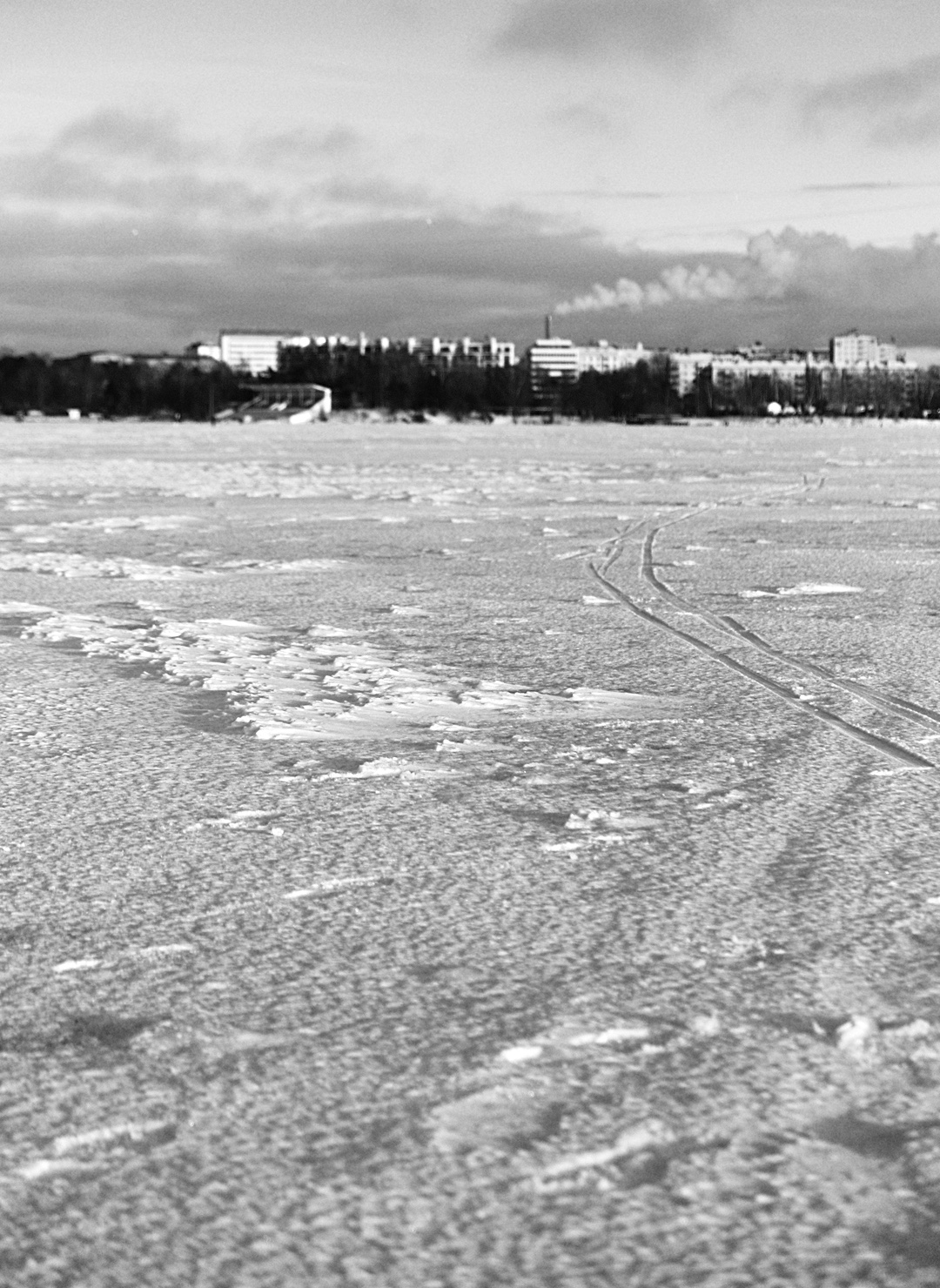
A picture of freezing Helsinki, taken from the ice covered sea.
Next, we need a signal which we will quantize. We can use the image’s luma, \(l\), which is a weighed sum of the image’s \(R\), \(G\), \(B\) components. This signal is typically associated with the “black and whiteness” of an image. Even though the original image is already black and white, the pixels still contain all three RGB values. Using luma in our code enables us to also use color images as input for our dithering algorithm, and still produce sensible output images.
Finally, we need a threshold value, a number which chooses whether a luma value is converted into black (0.0) or white (1.0). Choosing 0.5, we obtain the following step function for each pixel \(p_{x,y}\).
Running our image through this function with using gives us the following result.
Not a very good looking result. Luckily, we already know that we can do better than this!
Dithering
The dithering algorithm is based on the quantization algorithm above and requires just one modification to it: it adds noise to the threshold values. This has the effect of distributing the harsh boundaries between black and white in the quantized image. The classical way of distributing noise is by using Bayer matrices.
Bayer matrices
A Bayer matrix, \(M\), looks like this.
The matrix is square and is characterized by its side length \(N\) which in this case is 4. The matrix consists of elements \((0,;1,;\ldots,;N^2-1/N^2)\) which are distributed in such a way that the distance between elements of the sequence is as large and as even as possible across the matrix. We can generate a Bayer matrix for side length 2, 8, or 16 as well. The last section of this post contains notes on how you can generate your own Bayer matrix.
For any given pixel coordinate \((x,,y)\) in our image, we can map the pixel coordinate to the Bayer matrix element \((i,,j)\) using the modulo operator: \((i,,j)=(y,\text{mod},N,;x,\text{mod},N)\). The idea is to use the matching Bayer matrix element as the threshold value while doing quantization, instead of just a single number like 0.5. Inserting the Bayer matrix element into the previous step function, we obtain
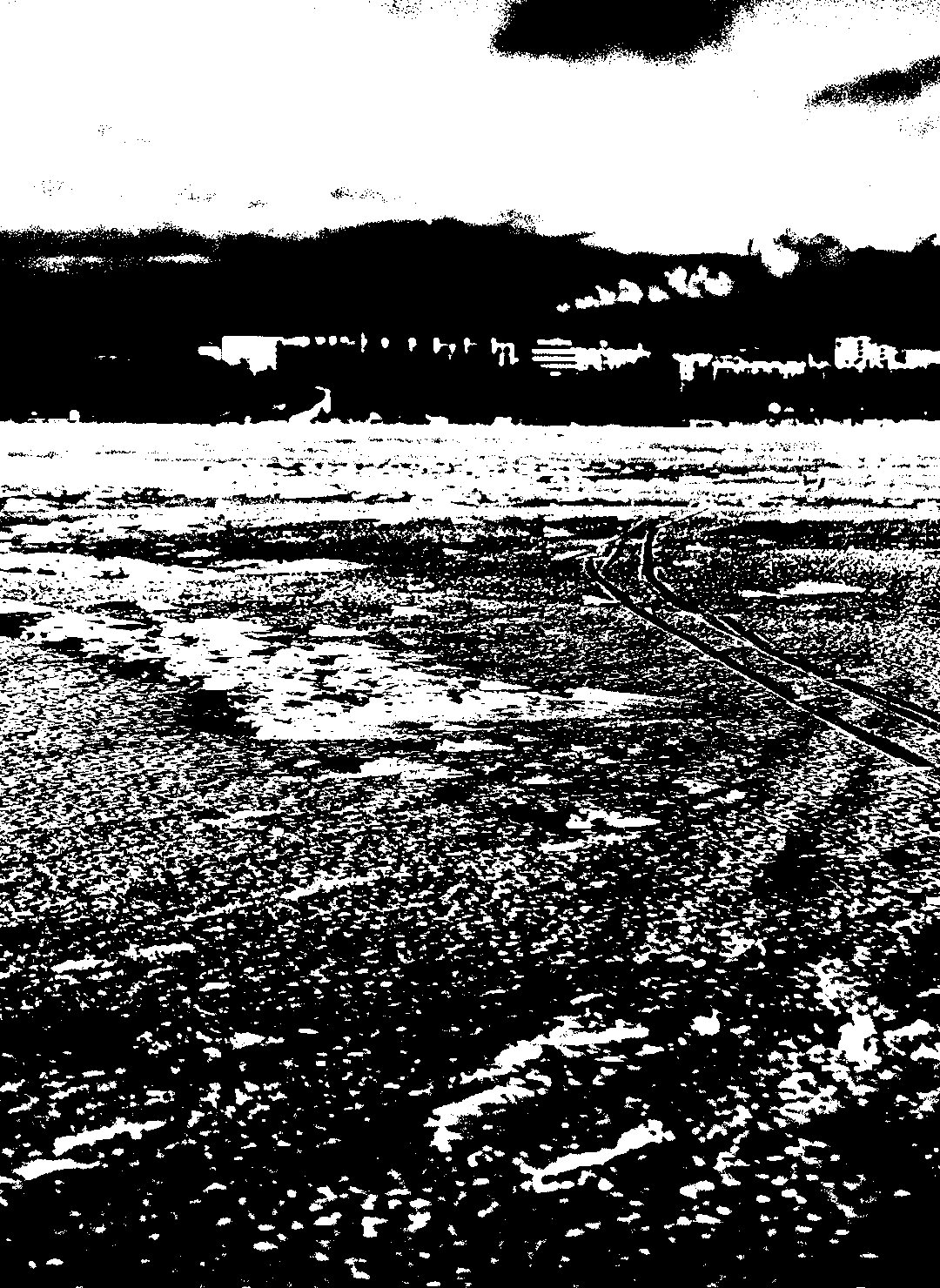
Running our image through this function using \(N=4\), we obtain the following result.

The landscape dithered with a \\(\mathbf{M}_4\\) matrix.
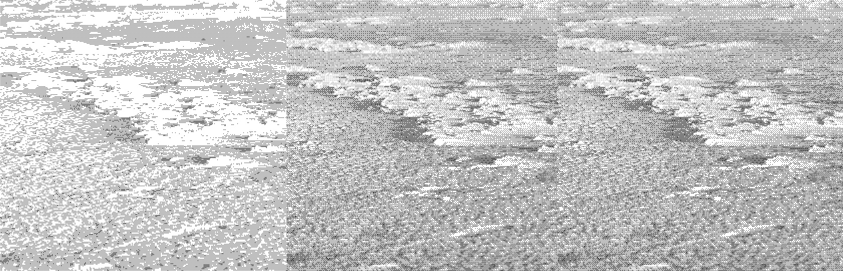
The details of the original image are now clearly visible, although we do have a visible grid-like pattern. We can dither with Bayer matrices using \(N=2,8,16\) as well.
Snow detail with \\(N=2,8,16\\) respectively.
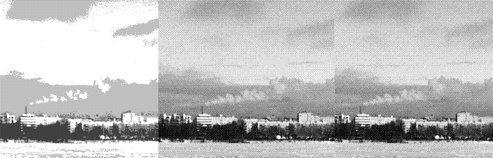
Sky detail with \\(N=2,8,16\\), respectively.
Looking at the image dithered using \(N=2\), we can still see detail resembling the original images in places of finer detail, such as the snow banks. But in places where finer gradients exist, such as the sky, the result is closer to the original naive quantization. There is almost no perceptible difference between the images dithered using \(N=8\) and \(N=16\). Comparing the sky using \(N=4\) and \(N=8\), you can see that there is clearly more detail using \(N=8\). That is where the sweet-spot between detail and matrix size seems to lie.
Although the results using larger Bayer matrices look good, there is just no way of getting rid of the slight crosshatch artifact, arising from the deterministic way the values are distributed. Our next two dithering methods will attempt to get rid of the pattern, by introducing randomness.
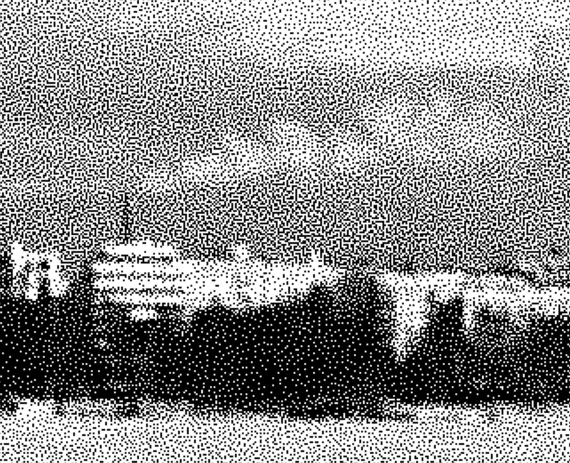
Random noise
The simplest way to add some randomness to the threshold value is to replace the Bayer matrix lookup with a call to a uniform random number generator.
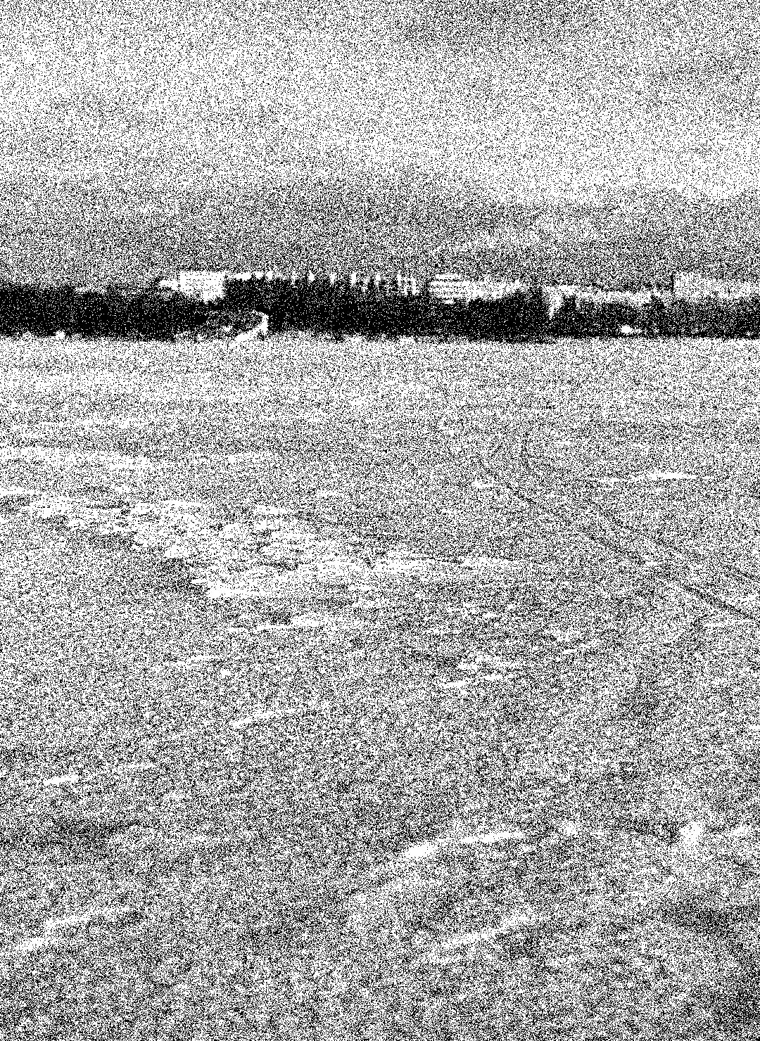
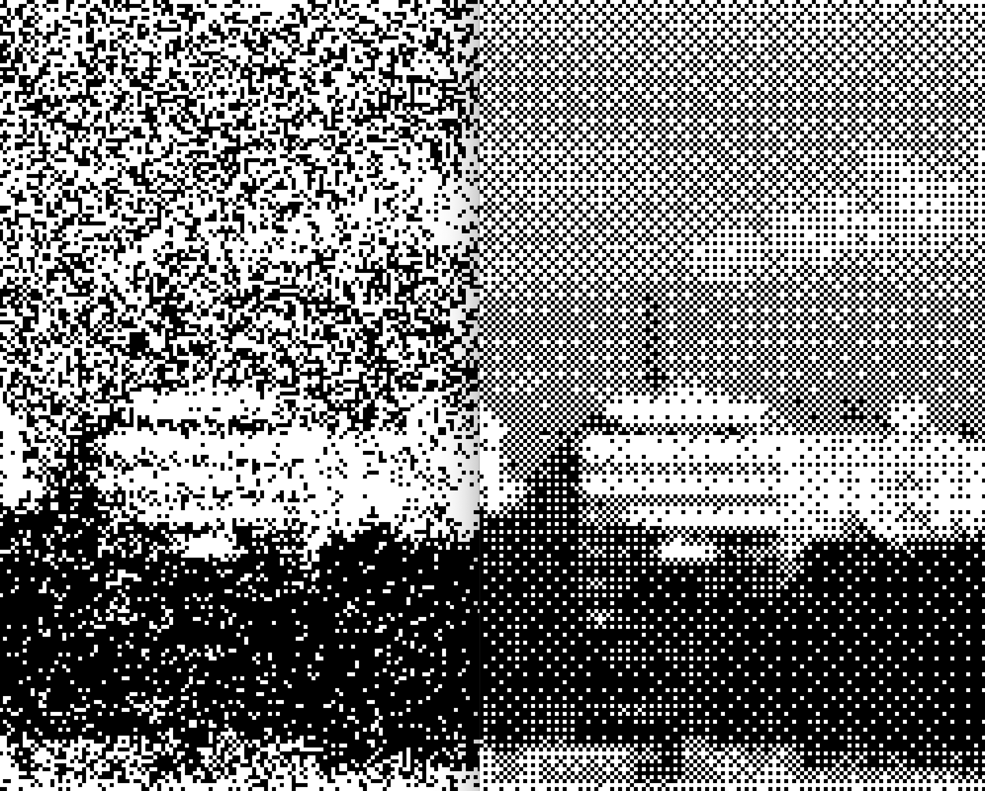
While we no longer have any visible crosshatch artifacts, the image has even less detail than in the previous section. Unlike the Bayer matrix, where neighboring values are guaranteed to be distributed evenly about the matrix, we can obtain multiple similarly valued uniform random numbers in sequence. As a result, our image loses detail due to the clustering of black and white. Nowhere is this more visible than when comparing the white plume from the smokestack with the images dithered with a Bayer matrix.
Blue noise
Blue noise is going to come to the rescue and restore the detail that we lost with the random noise. Blue noise values, like the random numbers used in the previous section, are distributed uniformly. But the frequency distribution of blue noise is different. Blue noise has less low-frequency components than the random numbers used in the previous section. Subsequent random numbers are more evenly distributed from each other.
This is what blue noise values look like in an image.
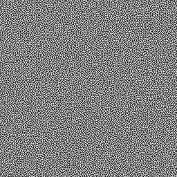
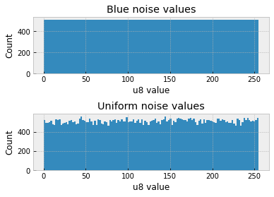
If we were to blur this image, it would look uniformly gray. This is the reason images look better when dithered with blue noise. We can verify that the pixel value distribution in blue noise is uniform by comparing it against uniform random numbers in a histogram.
Blue noise image masks, like the one above, are very expensive to compute. I used a free texture obtained from http://momentsingraphics.de/BlueNoise.html. These textures can be tiled, meaning that patterns due to repetition should be impercetable.
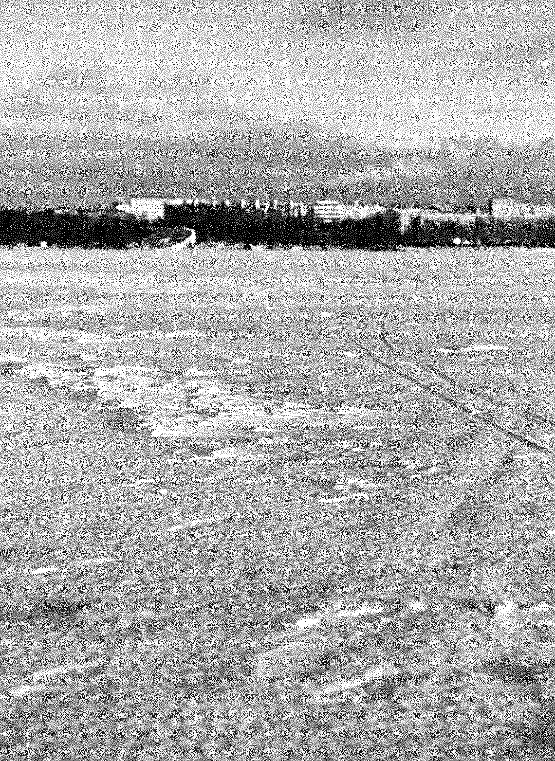
You can use the blue noise image mask exactly like a Bayer matrix. Load the pixels into a large matrix, and map pixel coordinates \(x\), \(y\) to image coordinates \(i\), \(j\) using the modulo operator. The resulting dithering function is exactly the same as the Bayer dithering function. Doing so, we obtain the final image, which was also the first image shown in this post.
Looking at the sky and snow detail, we are able to resolve far more detail than before, by simply adjusting the spatial distribution of our black and white pixels.
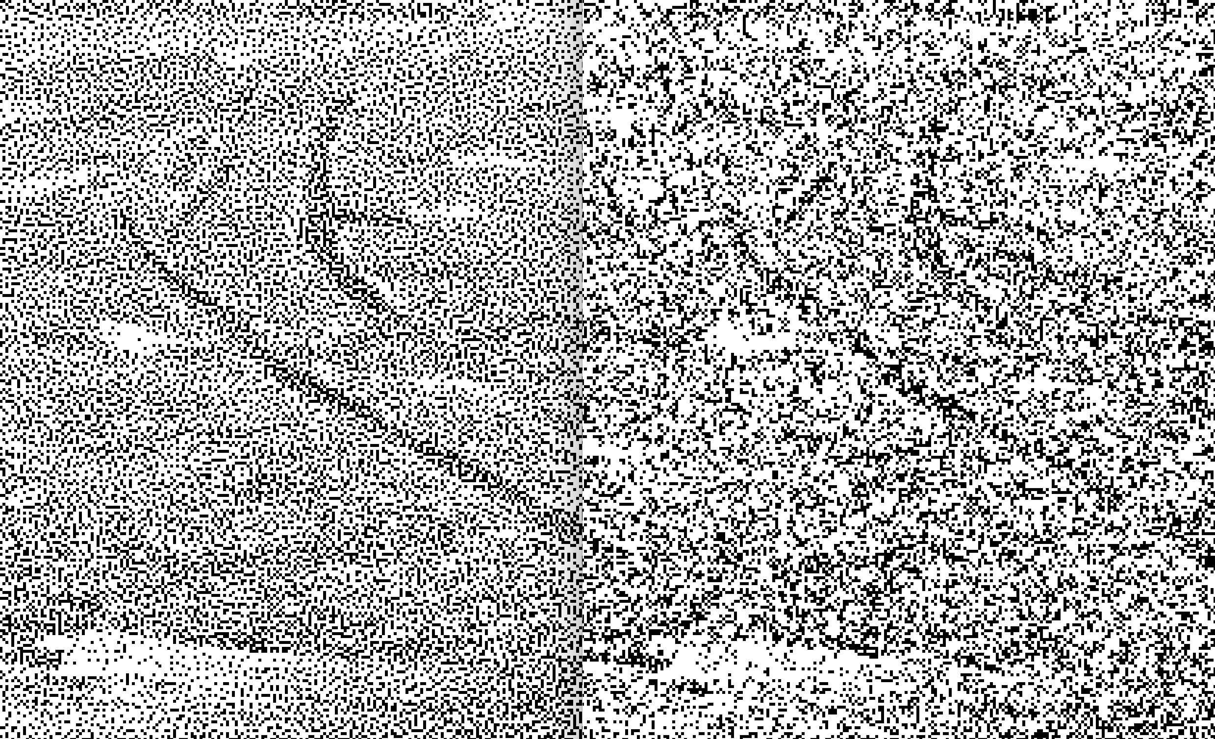
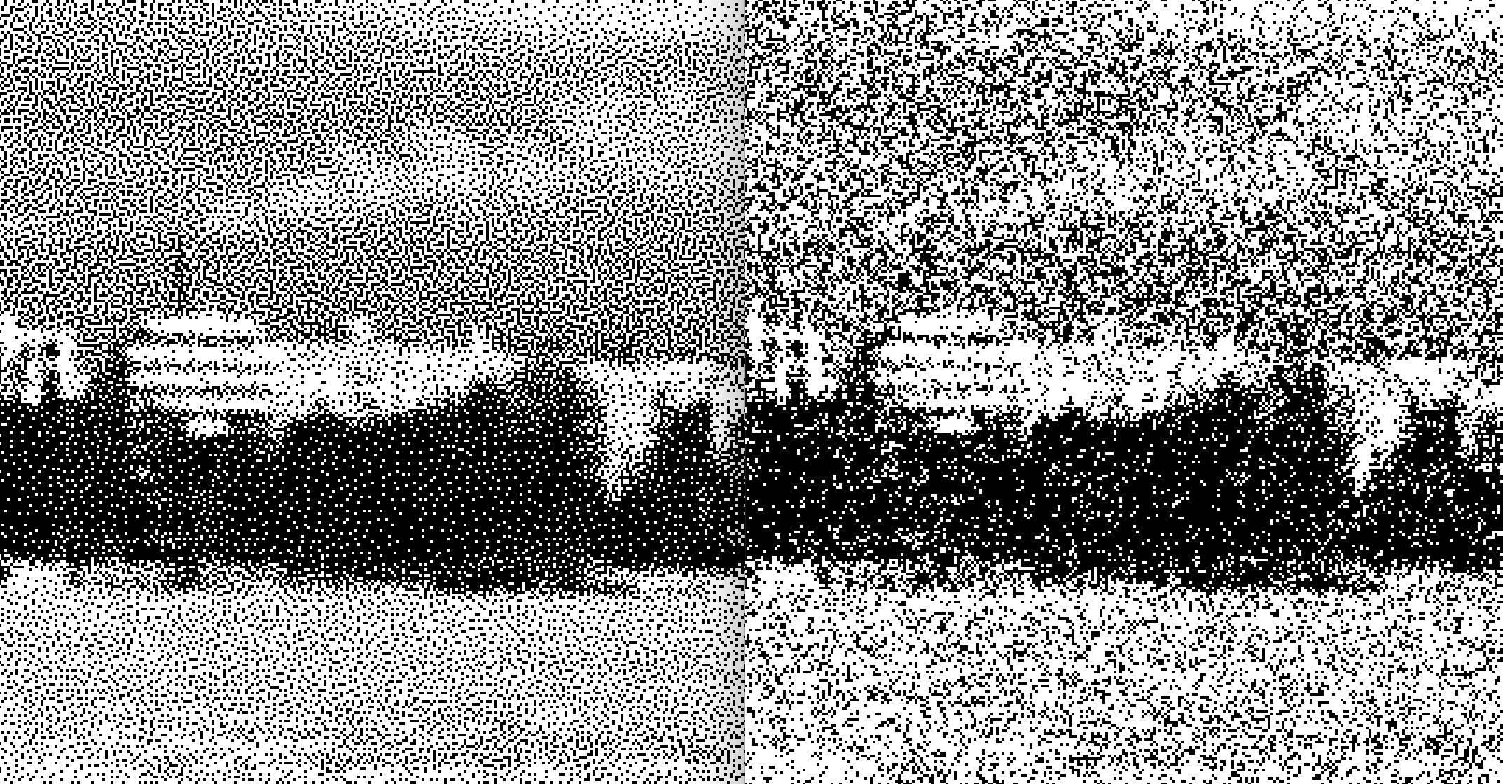
Blue noise on the left, random noise on the right.
Implementation notes
Using the https://crates.io/crates/image crate, it’s remarkably easy to load, transform and output images. You can obtain a black and white image with two lines of code.
|
|
With just a few more lines of code, it’s possible to transform, and output a result. This is a really fun way to get familiar with Rust.
Dithering function
Having loaded an image, it’s time to run its pixels through a dithering function. The dithering function uses a ThresholdMatrix struct and applies it to each pixel using the step function for Bayer dithering seen earlier. All dithering methods in this post are implemented using matrix look ups.
|
|
The ThresholdMatrix is a matrix containing luma offset values, with dimensions nx and ny.
|
|
In order to implement the different dithering methods, all we need to do is to initialize the matrix with values in three different ways. The next sections adds associated functions to ThresholdMatrix to do just that.
Bayer matrix
Generating Bayer matrices is perhaps the most interesting part of the implementation. Starting from Wikipedia, we could just hard code the matrices presented in the article. But what if we want larger matrices than \(N=8\)? In that case, we need to generate our own matrices of arbitrary size.
Wikipedia mentions two ways of generating your own Bayer matrix: a recursive algorithm, and a matrix elementwise bit manipulation algorithm.
On the surface, the elementwise algorithm seems simpler to implement in Rust. However, the Wikipedia article seems to have misunderstood the meaning of the source. It says that you can bit reverse the bit interleaved values x ^ y and y. However, in the original source, Joel Yliluoma’s arbitrary-palette positional dithering algorithm, the bits are interleaved in reverse:
|
|
This is not quite the same as bit-interleaving xc, y, and reversing the bits of that. Doing so would give you really large integer values, closer to the maximum value of the integer than to \(N\).
The Rust version of this algorithm isn’t totally straightforward, since there are a few C things which can’t just be copy-pasted over.
|
|
Random noise
Random noise is implemented by generating \(x\times y\) random numbers and storing them in the matrix. \(x\) and \(y\) need to be the image dimension in order for this to work.
|
|
Blue noise
Finally, blue noise is “generated” by loading the blue noise image into the matrix.
|
|
References
https://en.wikipedia.org/wiki/Ordered_dithering
Joel Yliluoma’s arbitrary-palette positional dithering algorithm
Image quantization and plots were done using Python.