Halton sampling
2026-09-08
Commit: cdd5249
Basic Halton sampling is implemented. Each pixel (stable stream, e.g. a pixel index) and dimension gets its own stream of Halton values, via a rotation hash:
|
|
It effectively rotates the sequence of hashed values in a unit circle. Averaging neighboring streams yields white noise. But within a stream and dimension a stable Halton sequence is obtained. A sequence of 2d or 3d values can then be generated:
|
|
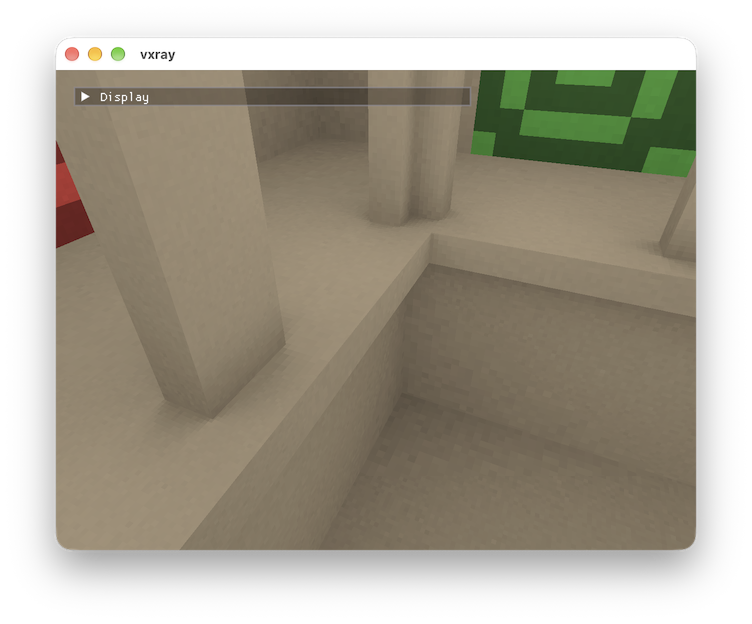
Here is the AO baseline with 2000 samples:
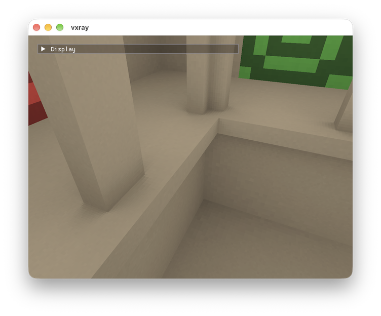
The same number of samples with Halton sampling:
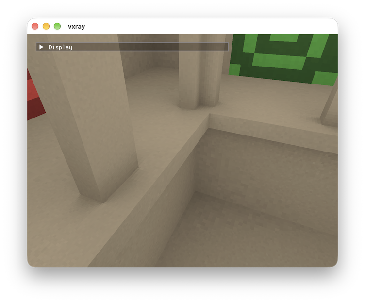
Baseline results are obtained with roughly half (1000) the number of samples:
Wavefront path tracer with spatial hashing
2026-09-06
Commit: c04e743
A wavefront path tracer with spatial hashing is implemented. The path tracer samples lambertian normals and the sun disk using single-sample MIS:
$$ F = \frac{f(X)}{{(1/2)p_1(X) + (1/2)p_2(X)}} $$
where the direction sample X is sampled from either the cosine-weighted normal distribution of the sun disk distribution with a probability of 1/2.
The wavefront path tracer is loosely based on Jacco Bikker’s blog entry. It contains the following steps:
- Generate: for each pixel in a gbuffer raster, generate a path and scatter rays using MIS and place them into the ray queue.
- Extend: intersect each ray with the voxel grid using sparse ray marching. Also shade each intersection by updating the path’s throughput and place the scattered ray (if there was one) into the output ray queue.
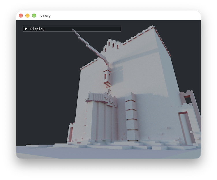
- Accumulate: for each path, outputs the albedo demodulated radiance into the spatial hash using the path’s radiance.
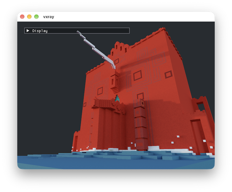
To display a path traced image, the shading from the spatial hash has to be multiplied by the albedo again. This retains the surface details which would otherwise be lost due to the averaging which happens inside each spatial bucket.
The albedo-demodulated radiance stored in the spatial hash map.
The remodulated radiance gives the final result.
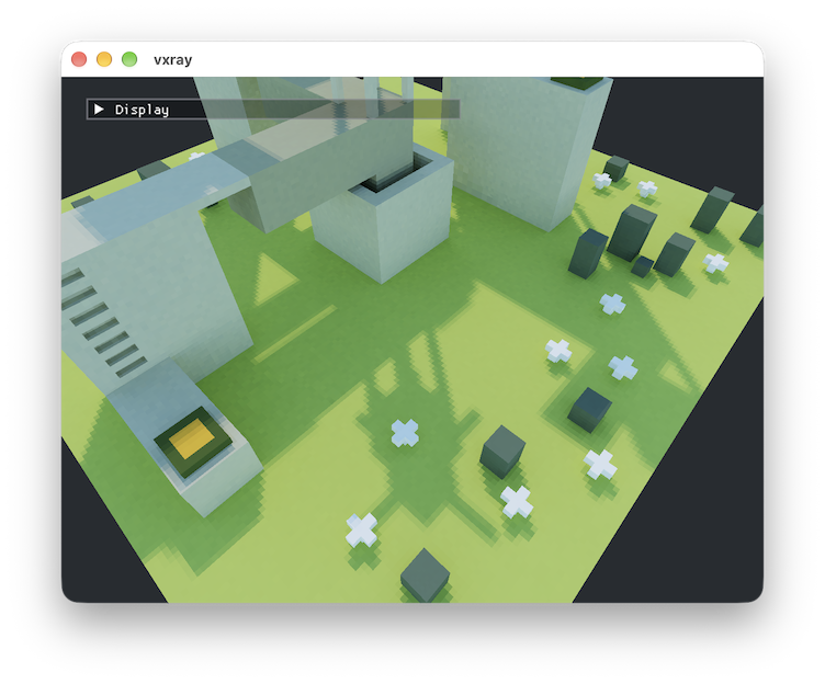
Like the AO shading earlier, large cell sizes give a blocky look. This image, however, does not contain any spatial filtering.
Sky view LUT
2026-09-02
Commit: 4be4ee7
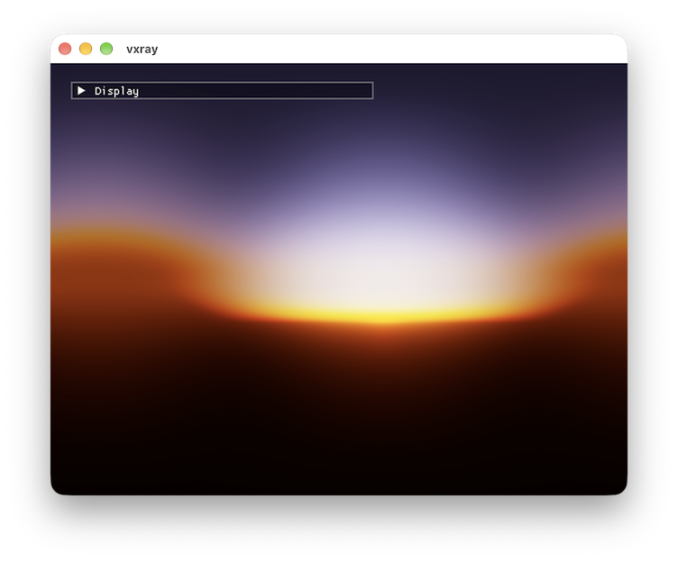
The raymarched atmosphere shaders from github.com/Fewes/MinimalAtmosphere are ported to vxray. The sky view LUT with angular compression is implemented from Seb Hillaire’s A Scalable and Production Ready Sky and Atmosphere Rendering Technique.
Here is what the 400 x 400 LUT looks like. It is rendering a sky at an altitude of 20 km, with sun just below the planet’s horizon.
Reproject spatial hash map indices
2026-09-01
Commit: c41b366
Splits the RTAO pass into two steps:
- Hash indices from the previous frame are reprojected to the current frame if the history and checksum is valid. The hash index is looked up otherwise. The current frame’s hash index is written to a texture.
- A fullscreen RTAO pass is done using the gbuffers and the hashmap index texture.
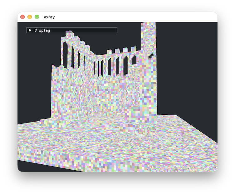
A view of the index texture
The intention is again to try reduce the impact of the spatial hash lookup. I tried splitting the spatial hash lookup into a separate pass to improve shader occupancy, but looking up the index and rendering it to a texture was taking over 6 milliseconds on a Macbook Air (M2). See the highlighted pass from the Metal debugger:
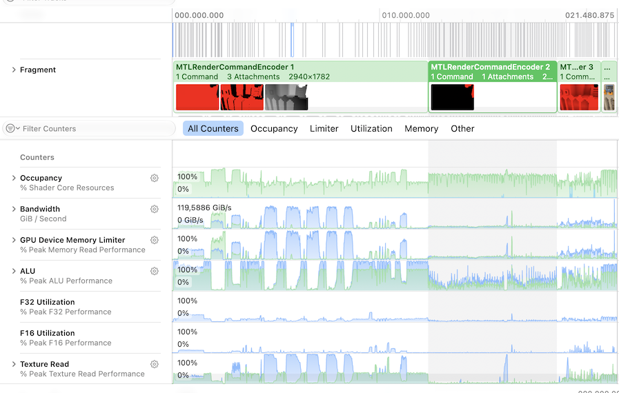
There is higher MMU activity during the index pass than for other passes. From the memory counters:
- Last Level Cache Miss Rate: 8.31 % (much better than the other render passes!)
- Device Atomic Bytes Read: 309.19 MiB
- Device Atomic Bytes Written: 617.13 MiB
It seems that the atomic reads and writes used to write to the hash map data structure does come with a penalty.
By reprojecting the indices from the previous frame and only going down the code path with the atomic reads and writes if the history is invalid or there is a mismatching checksum, the index pass duration is reduced to 2 milliseconds. The memory counters now say:
- Device Atomic Bytes Read: 4 KiB
- Device Atomic Bytes Written: 19.16 MiB
Even if a valid hash entry is reprojected, the frame counter has to be updated atomically. But it doesn’t have to be updated every frame:
|
|
Performance numbers:
monu2.vox
| Metric | Before | After | Uplift |
|---|---|---|---|
| FPS | 144.00 | 143.90 | −0.07% |
| Average GPU walltime | 6.46 ms | 5.88 ms | −9.01% |
sponza-1024.vox
| Metric | Before | After | Uplift |
|---|---|---|---|
| FPS | 64.81 | 67.72 | +4.49% |
| Average GPU walltime | 26.17 ms | 24.95 ms | −4.68% |
OK, it’s not a night-and-day difference, especially in the heavy Sponza scene with a billion voxels, but it’s good to know the renderer isn’t doing 6 milliseconds of work that it doesn’t need to.
Sparse ray marching with axis-aligned distance fields
2026-08-25
Commits:
The existing DDA renderer is completely rewritten. A sparse raymarcher, using nested axis-aligned distance fields (NAADFs) is implemented, inspired by Globally Illuminated Voxel Worlds Accelerated with Nested Axis‐Aligned Distance Fields. Brick coordinate rasterization is removed in favor of a simpler pipeline. This method seems like a really promising way to implement both the basic gbuffer + RTAO rendering, as well as a potential path tracer.
The three-level grid from the NAADF paper is adopted, with the existing bottom level voxel grid, a brick grid with each brick containing 4³ voxels, and a chunk grid with each chunk containing 4³ bricks.
An axis-aligned distance field is a grid, where each cell contains six distances, two per axis. The distances are the number of free cells along the axis. An AADF is computed per grid. Naive axis-aligned distance fields are computed, i.e. the grid compression method from the paper is not implemented. This means that empty space, especially at the voxel grid level, contains significant redundancy. For a 1024³ voxel grid, the voxel AADF alone weighs 4 GiB, which means that this is not av ery scalable method in its current form. But for smaller 256³, such as the grids in my Polycube voxel editor, the AADF weighs only 64 MiB.
Traversal is similar in spirit to DDA, but instead of stepping across one cell boundary each step, we step over the largest empty space, calculated from the AADF. The RTAO shader is a simple way to demo the method, as it performs a ray march only at the voxel grid granularity:
|
|
The performance regresses a little bit compared to earlier in both small and especially larger scenes on a Macbook Air (M2). The ability to render sponza-1024.vox, with 1 billion voxels and ray tracing, at 60 FPS on a large monitor is still impressive, given the relative simplicity of the rendering pipeline.
monu2
| Metric | Before | After | Uplift |
|---|---|---|---|
| FPS | 144.00 | 144.05 | +0.03% |
| Average GPU walltime | 5.11 ms | 6.35 ms | +24.30% |
sponza-1024
| Metric | Before | After | Uplift |
|---|---|---|---|
| FPS | 81.41 | 64.73 | −20.48% |
| Average GPU walltime | 20.72 ms | 26.28 ms | +26.86% |
The occupancy of the gbuffer pipeline is much better now:
- FS Occupancy: 52.02 % (up from 40.13 %)
- Register allocation: 60 (down from 76)
But I inadvertently tanked the performance of the RTAO shader in commit f332529 by introducing a loop around the sparse ray march:
- FS Occupancy: 36.38 %
- Register allocation: 82 (up from 55)
That is to be fixed in a future commit.
Merge RTAO pipelines
2026-08-22
The compute and pixel shaders are merged into one pixel shader. Earlier, a compute pass was introduced, which accumulated samples into the spatial hash using a screenspace checkerboard pattern. This was done to reduce the impact of the spatial hash lookup. It turned out that just a single simple per-pixel sample in a pixel shader was actually faster overall.
FPS jumped from 74 to 80.
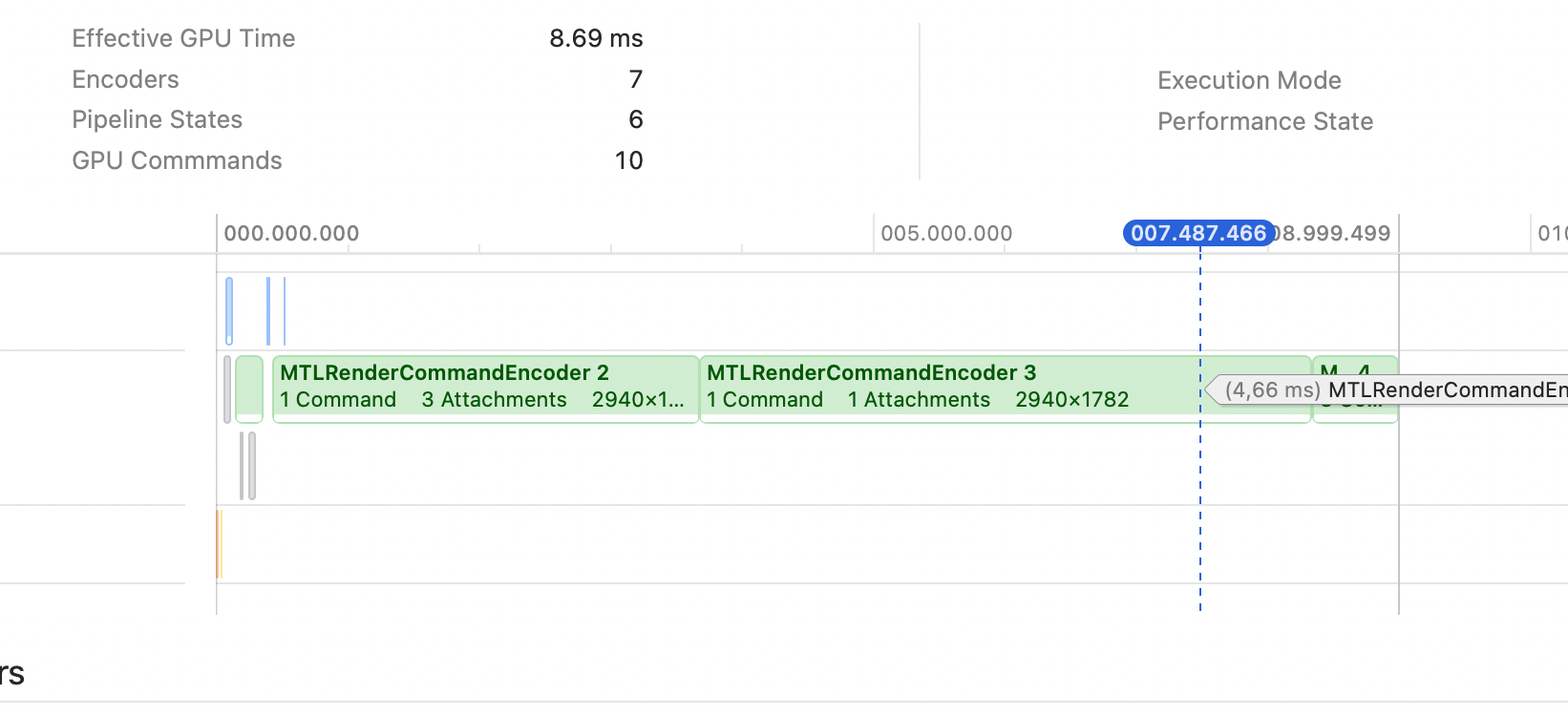
Before: both the compute and render pass accumulate to roughly 5 ms.
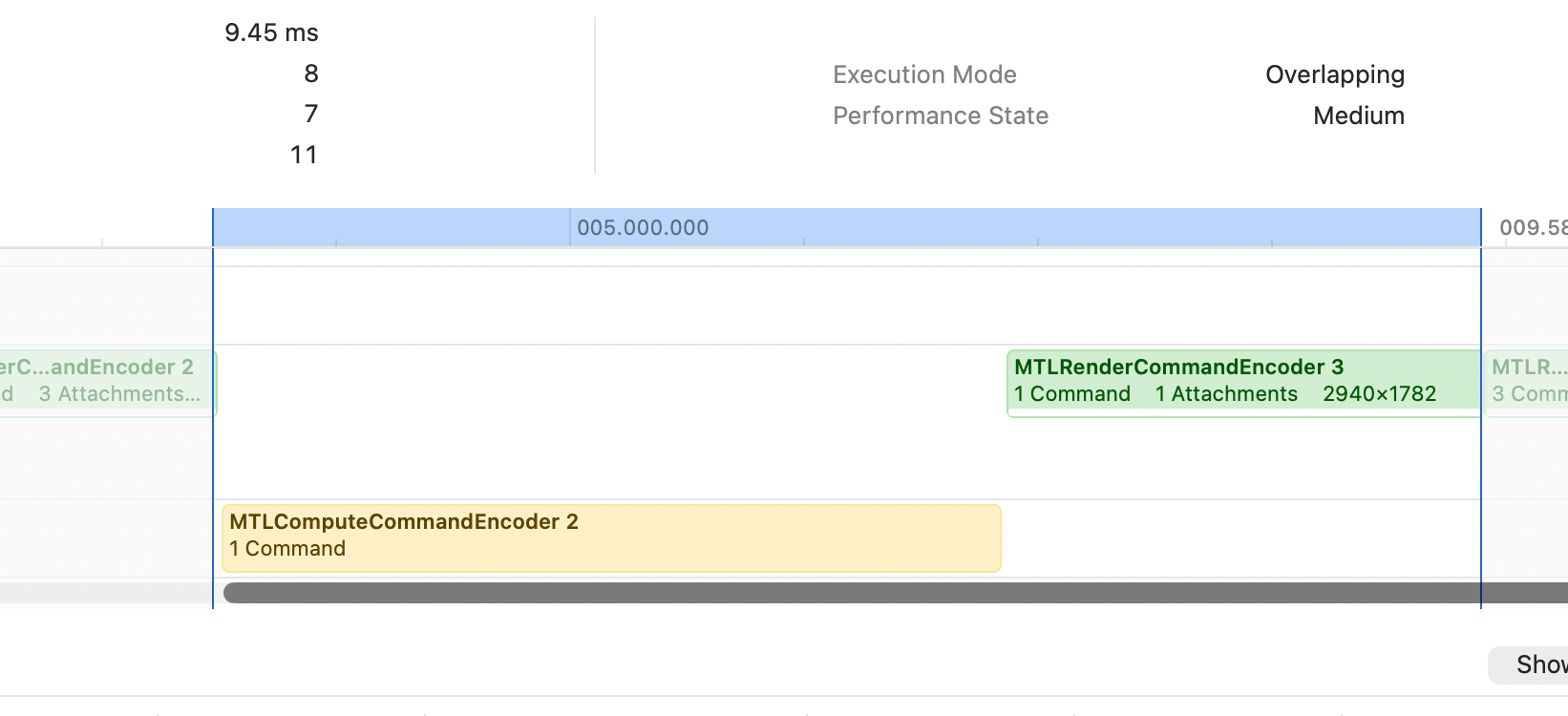
After: a single pixel shader was slightly faster.
Experiment: Atrous spatial filtering
2026-08-18
Commit: 8a67b2d
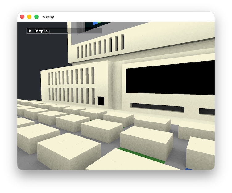
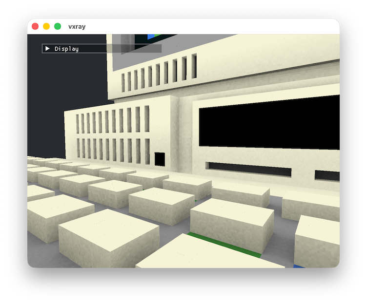
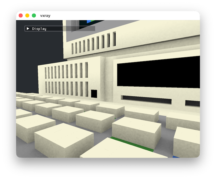
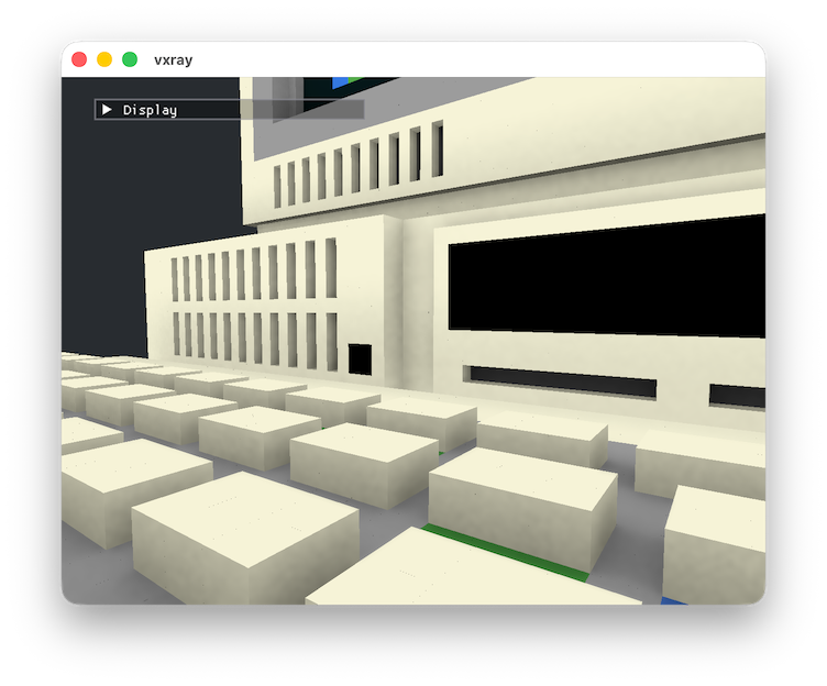
Experimental spatial filtering is implemented using Atrous wavelet filtering. This update is for posterity, as the performance was so terrible that this change is reverted.
Atrous filtering works in iterations. Each successive iteration increases the filtering radius.
|
|
Baseline
1 iteration
2 iterations
3 iterations
4 iterations
4 iterations of atrous filtering removes visible noise, and even allows further increasing the cell size to 16 with very little visual impact. Unfortunately, running a single iteration took almost half as long as all the rest of the rendering combined (8 - 10 ms). 4 iterations made the rendering a slide show.
I am not intersted in heavily optimizing spatial filtering now, so this change is reverted. I will embrace the slightly blocky visual artifacts of spatial hashing.
This is my kernel. My edge-stopping function accounts for normals and depth. The depth term is borrowed from the SVGF literature.
|
|
Shader optimizations
2026-08-17
Commits:
This update contains three commits which improve performance.
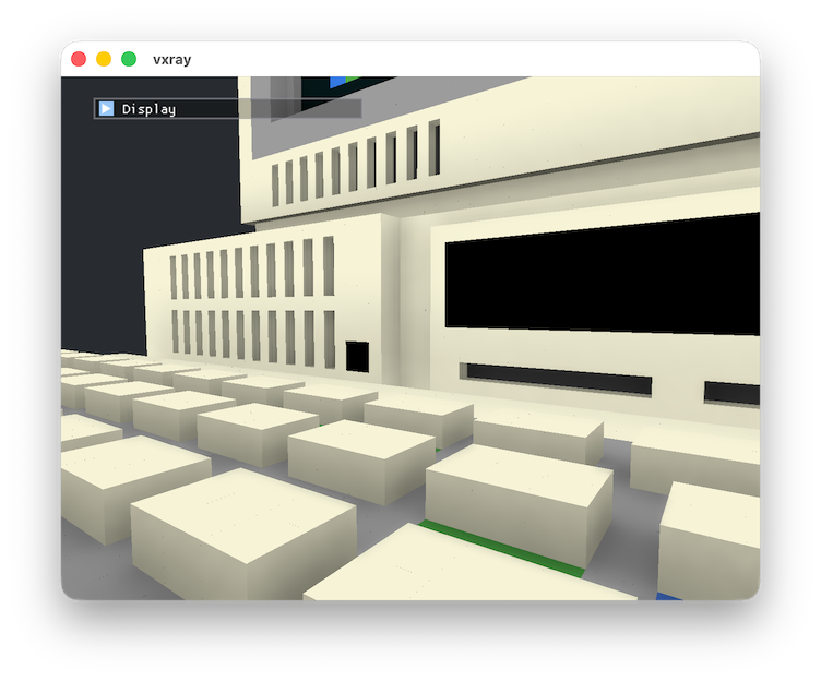
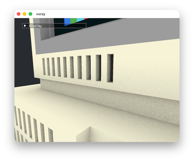
Increase cell size from 5 to 10. Increasing the cell size means fewer resident hash map entries, with more pixels contributing to the value of the hash map entry (collaborative ray tracing, faster cell convergence). This change has a noticeable visual impact, although on a retina monitor it’s not a huge difference.
Cell size 5
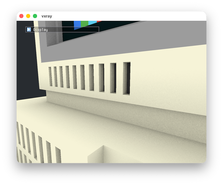
Cell size 10
Update spatial hash map using a checkerboard pattern. Instead of mapping each pixel of the gbuffer to a spatial hash map cell, only every other pixel is mapped to a cell and sampled for RTAO. Two RTAO samples are per pixel, to keep the same overall RTAO sample count. On alternating frames, the pixel pattern changes to cover all pixels. The motivation of this change is to reduce the impact of spatial hash search + update.
Frame 0:  X . X .
          . X . X
          X . X .

Frame 1:  . X . X
          X . X .
          . X . X
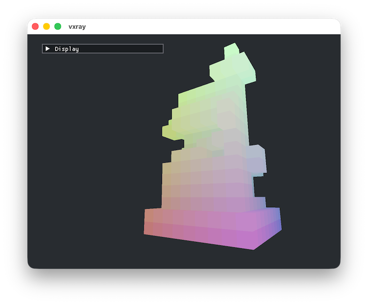
Rasterize brick coordinates. The rasterized brick AABB depth is replaced with rasterized brick coordinates. The somewhat complex code to reconstruct the brick position from the depth buffer was completely removed, and the brick coordinate is passed straight to the DDA algorithm.
Before:
- FS Occupancy: 34.30 %
- Register allocation: 89
After:
- FS Occupancy: 40.13 %
- Register allocation: 76
A visual of the rasterized brick coordinates
The performance was again measured in sponza-1024-1 on a Macbook Air (M2).
| Configuration | FPS | GPU walltime |
|---|---|---|
| Baseline | 39.04 | 46.16 ms |
| Cell size 5 → 10 | 71.73 (+83.72%) | 23.50 ms (−49.10%) |
| Checkerboard spatial hash update | 71.96 (+84.33%) | 20.03 ms (−56.60%) |
| Rasterized brick coordinates | 72.00 (+84.42%) | 19.33 ms (−58.12%) |
The improvement compared to before is significant, with the largest improvement coming from the increase in cell size! The overall frame rate is still much lower than the previous best (137.20) at the same scene and view, but that was measured while rendering only the albedo. The renderer is doing a lot more now.
Performance interlude 2
2026-08-16
This update doesn’t contain changes to vxray.
While the spatially cached RTAO both looks better and improves performance, the performance on the Macbook Air (M2) is still not amazing when moving around the interiors of the Sponza scene compared to before.
A look at the Metal profiler timeline reveals that the RTAO hashmap update pass takes the most time during the frame. It also reveals that the gbuffer pass, which casts rays against the voxels, has a bloated register allocation of 89, up from 77. This has reduced the occupancy of the gbuffer pass to ~20 %. The change is due to a precision issue fix made in 870dbe8 which maintains a large number of float3s. Apparently large enough to increase the whole shader’s register allocation.
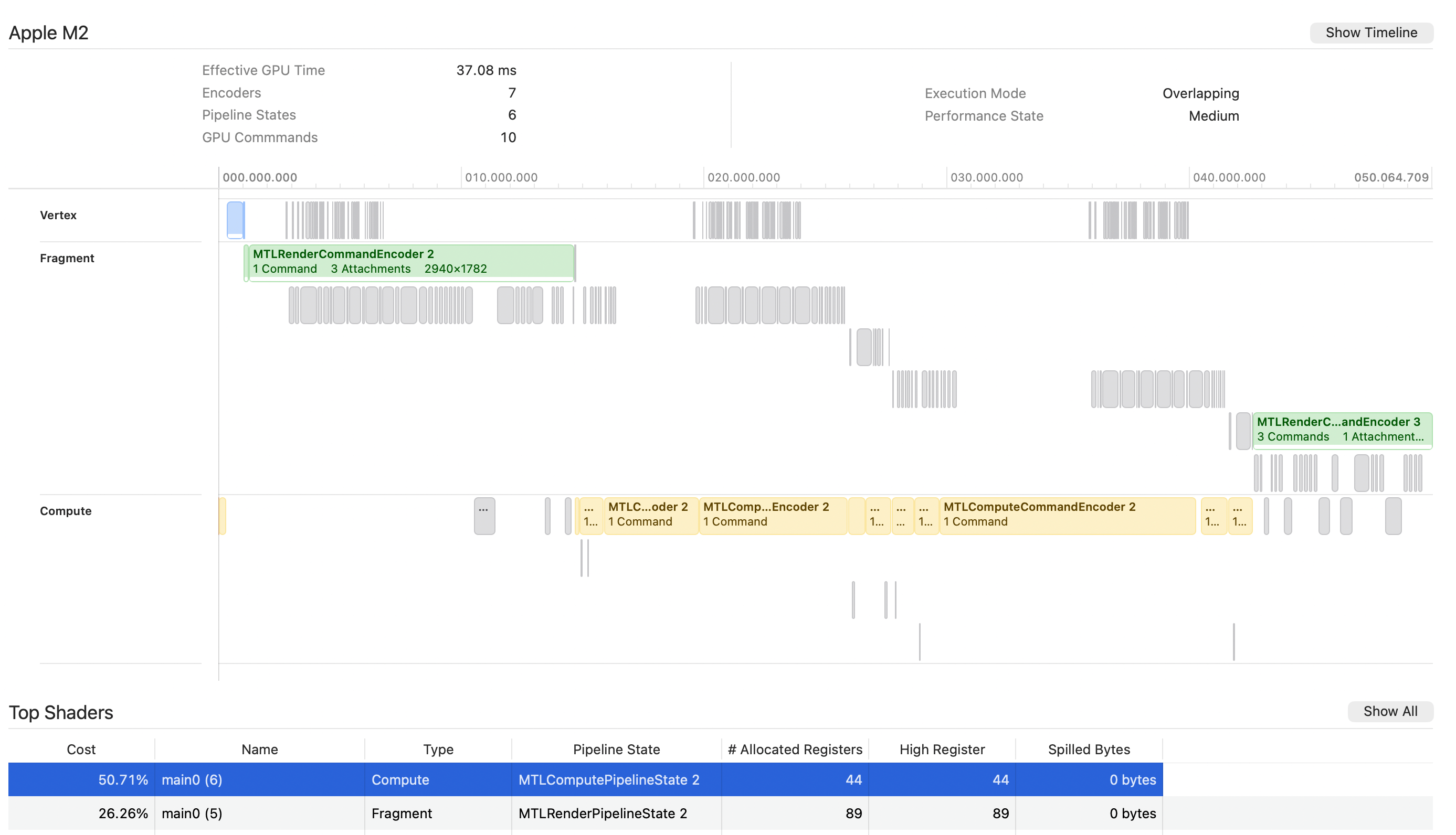
A look at the timeline reveals that, during the hashmap update, the memory unit is very active even though the memory bandwidth is not huge.
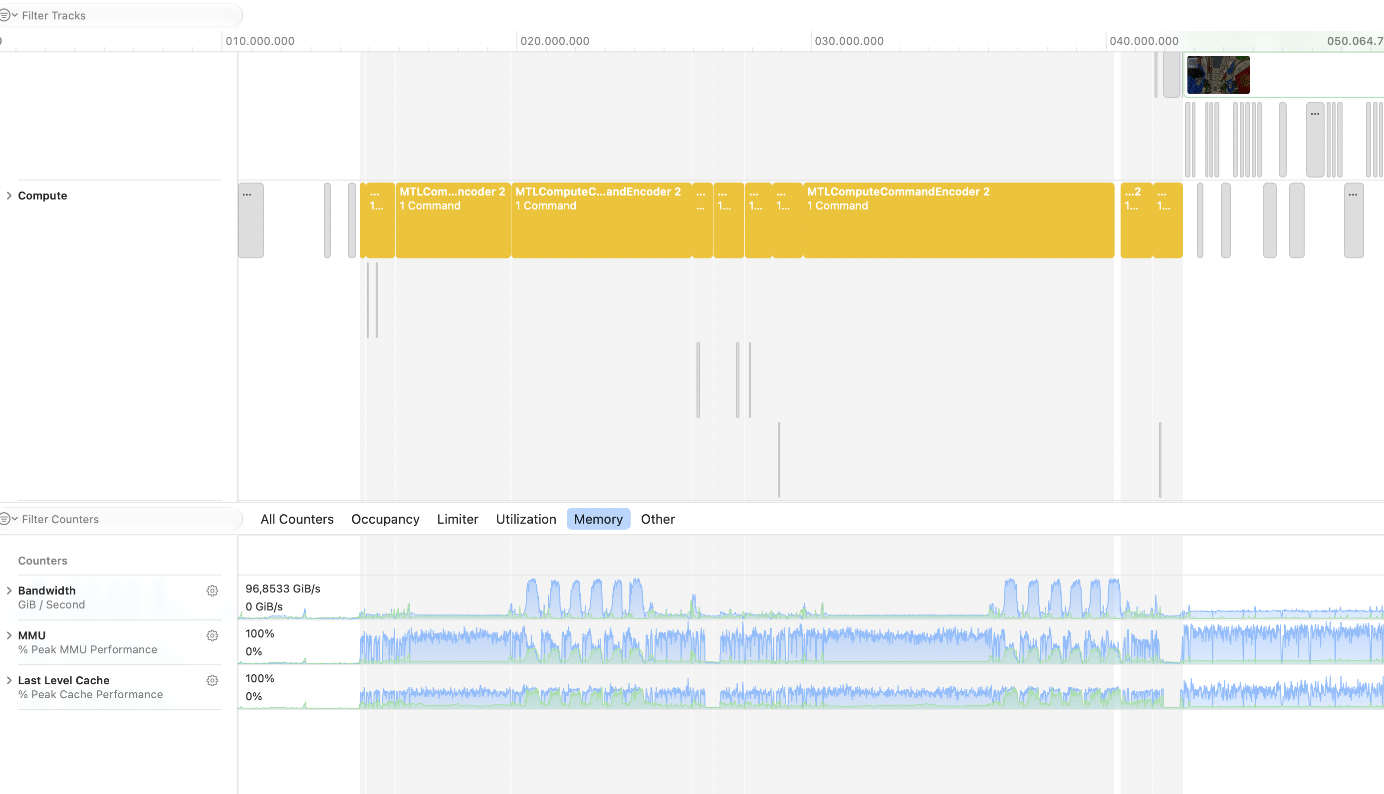
The hashmap lookup contains a number of atomic operations, which may have a bit of additional overhead compared to regular buffer reads.
|
|
For the next optimizations, the goal is to reduce the amount of times the hashmap is hit, as well as reduce the register allocation of the gbuffer pass to improve shader occupancy.
Spatially cached RTAO
2026-08-15
Commit: 4a6c4b7
Ambient occlusion values are stored in spatial cells in a hashmap, based on the method from Spatial Hashing for Raytraced Ambient Occlusion.
Since ambient occlusion is not view-dependent, it can be accumulated into a cell even if the camera moves without any reprojection.
The implementation follows the blog post closely, using the same parameters for cell size, cell age limit, and the same hash functions. The hash map size, however, was increased to 16 million elements to prevent running out of space when moving the camera around rapidly. At 4k resolutions, the algorithm was sometimes not able to find a free slot older than 20 frames.
Most of the code snippets from the blog post could be used almost verbatim. The code from the blog post is launched from a compute shader, which writes the occlusion count back into the hash map. The occlusion count and total sample count is fetched from the hashmap in a separate pass to shade the pixel.
|
|
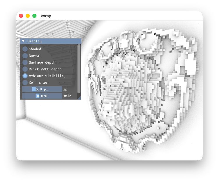
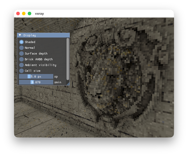
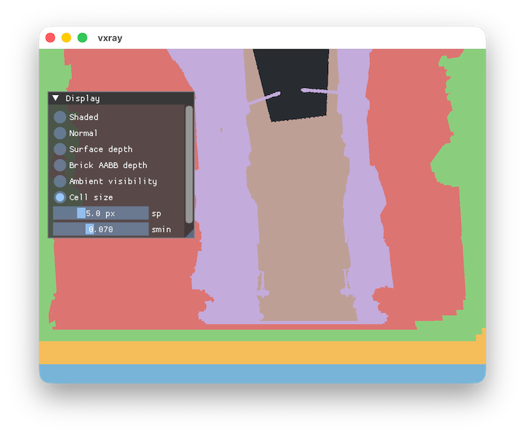
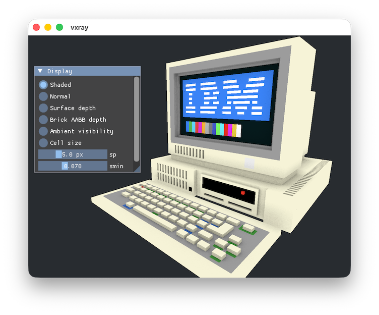
The cell size cascades are presented in this cell size visualization.
Naive RTAO
2026-08-13
Commit: 5087ab4
The ambient occlusion integral
$$ A(p) = \frac{1}{\pi} \int_{\Omega}V(p, \omega)(\mathbf{n} \cdot \omega)d\omega $$
is ray-traced using cosine-weighted hemisphere sampling. The method is explained in better detail in my other devlog.
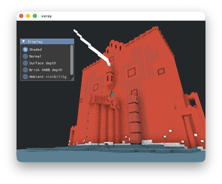
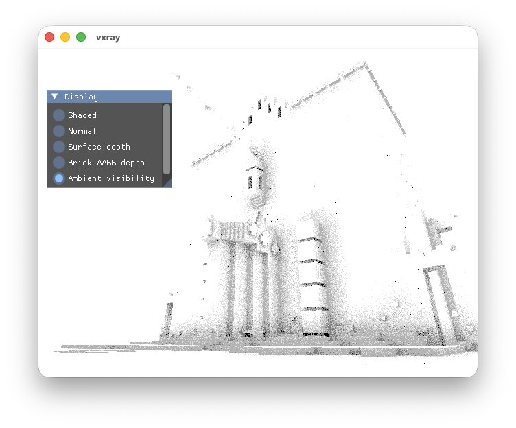
4 samples per pixel are used, with a radius of 8. No filtering or anything fancy is done at this stage. This has a major impact on performance.
|
|
Gbuffer pass
2026-08-12
Commit: 39ad989
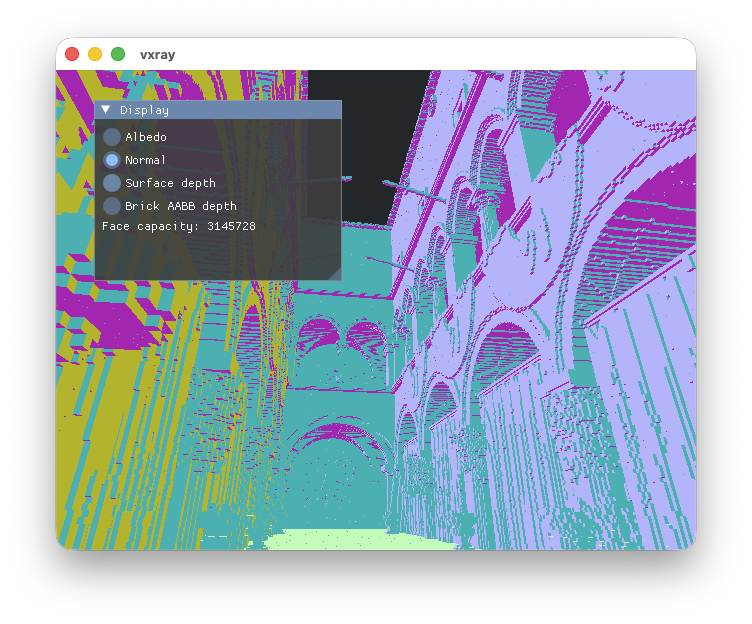
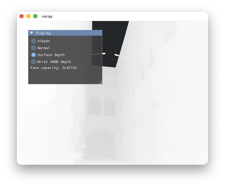
A gbuffer pass with albedo, normal, and depth targets is added. The depth is the rendered voxel depth, distinct from the AABB brick depth that we used to seed the DDA algorithm.
The gbuffer pass consists of two steps:
- Perform DDA as before, using the brick AABB depth as the starting point.
- If the DDA returns a voxel cell, then the ray is intersected with the voxel’s AABB.
The intersection step is performed outside of the DDA loop in order to prevent the register allocation of the shader from growing further.
Shader occupancy optimization 2
2026-08-07
Commit: 2975a50
Another optimization pass is done to the shader to improve occupancy. Grid cell coordinates are converted to int16 (since the largest possible grid extent is 1024) and the loop counters are eliminated.
Before:
- FS Occupancy: 36.05 %
- Register allocation: 88
After:
- FS Occupancy: 39.71 %
- Register allocation: 75
Additionally, ALU instruction count dropped by 10 %.
sponza-1024-1
| Metric | Before | After | Uplift |
|---|---|---|---|
| FPS | 111.59 | 137.20 | +22.94% |
| Average GPU walltime | 13.31 ms | 10.58 ms | −20.57% |
sponza-1024-2
| Metric | Before | After | Uplift |
|---|---|---|---|
| FPS | 142.99 | 142.66 | −0.23% |
| Average GPU walltime | 5.49 ms | 5.07 ms | −7.67% |
The improvement to the first scene is almost as large as the hybrid renderer update itself 🎉
Converting the branchless trick inside the loop to a big if-else eliminates the axis mask and further reduces the register allocation, but this made the framerate worse. The branchless trick is worth keeping.
|
|
Rasterize brick AABBs
2026-08-06
Commit: c5b6bf4
A hybrid renderer is implemented, significantly improving rendering performance. A billion voxels can now be rendered in real time 🎉 Each frame
- quads are generated for camera-facing brick faces
- the brick quads are rasterized into a depth buffer
- ray tracing uses the rasterized depth as the ray origin for DDA
Here is a visualization of the rasterized brick AABB depth buffer along with the final render using ephtracy’s monu9.vox from ephtracy/voxel-model.
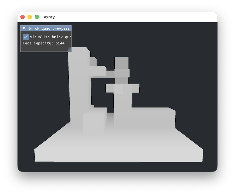
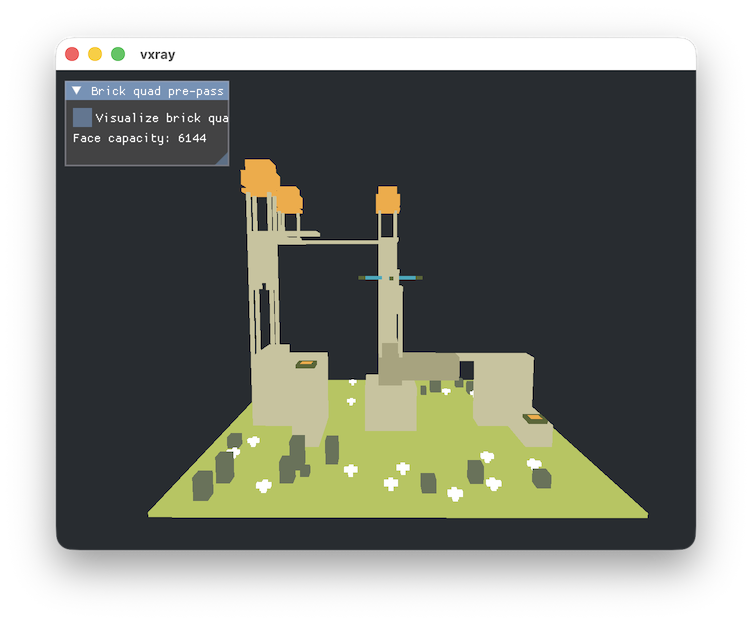
Rasterized brick AABBs allow skipping over empty space much faster than traversing through bricks with DDA. While not necessary for rendering static models here, the quads are regenerated every frame to support dynamic voxel grids for future applications.
The higher-resolution 1024x1024x1024 voxelization of the Sponza Atrium scene is now used to measure performance. Measurements are done using a Macbook Air (M2), on a 3840 x 1600 144 Hz monitor.
sponza-1024-1
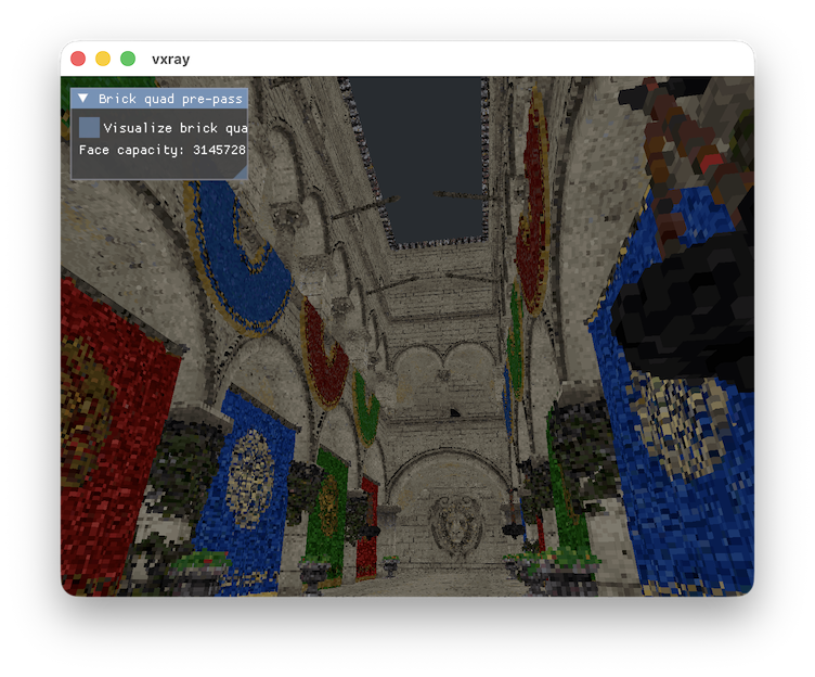
| Metric | Before | After | Uplift |
|---|---|---|---|
| FPS | 86.51 | 111.59 | +28.99% |
| Average GPU walltime | 18.51 ms | 13.31 ms | −28.07% |
sponza-1024-2
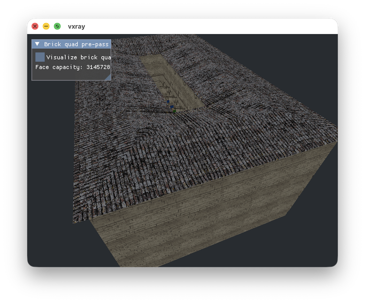
| Metric | Before | After | Uplift |
|---|---|---|---|
| FPS | 104.64 | 142.99 | +36.64% |
| Average GPU walltime | 14.42 ms | 5.49 ms | −61.91% |
Some notes on performance:
- when close to the model surface, a tighter fitting brick size (such as 4x4x4) improves performance
- when viewing the model from afar, a loose brick size (the current 8x8x8) is better
- rendering slows down significantly when looking along a surface inside a brick, as the DDA algorithm has to do the full brick + voxel traversal as before
Revert “Voxel occupancy mask”
2026-08-05
Commit: 8cb6aae
Reverts the previous change. It was cherry-picked from an exploration branch, and when systematically measuring the performance against the current parent commit, it performed worse in every scene. Oops.
The smaller brick granularity results in more bricks being visited along the ray, which slows down rendering especially when viewing the model from afar.
It performs better than the current implemention with VX_BRICK_EXT set to 4 in some scenes, so there may be merit to circle back to this idea in the future.
Voxel occupancy mask
2026-08-04
Commit: fdf44f3
The brick extent is reduced to 4x4x4. A voxel occupancy mask is introduced alongside the voxel grid:
|
|
Each brick contains 64 voxels. If we store voxel occupancy using a single bit, a single 64-bit integer is enough to store the occupancy of a single brick and quickly skip over the entire brick without an additional data structure:
|
|
trace_brick no longer needs to lookup occupancy in a texture, since it can now just use the voxel_mask value we loaded. If we find an occupied voxel along the ray, we can then look up the voxel grid and return the palette color:
|
|
Shader occupancy optimization
2026-08-01
Commits:
Fewer variables are carried over the loops and tdelta was deduplicated, reducing the register allocation by 20. In particular, using just the min cell inside both nested loops has a large impact:
|
|
The middle two commits clean up some unnecessary work. The occupancy metrics for the 2-level DDA shader improve significantly:
- FS occupancy counter: 42.37 % (up from 35.43 %)
- Register allocation: 72 (down from 92)
A modest occupancy bump! Here is how the renderer performs in practise on a Macbook Air (M2). This time, I measured the numbers on a 144 Hz ultrawide monitor running at 3840 x 1600:
monu2-1
| Metric | Before | After | Uplift |
|---|---|---|---|
| FPS | 143.20 | 144.00 | +0.56% |
| Average GPU walltime | 6.58 ms | 5.37 ms | −18.32% |
sponza-256-1
| Metric | Before | After | Uplift |
|---|---|---|---|
| FPS | 59.78 | 72.83 | +21.83% |
| Average GPU walltime | 28.39 ms | 22.51 ms | −20.71% |
sponza-256-2
| Metric | Before | After | Uplift |
|---|---|---|---|
| FPS | 109.53 | 143.94 | +31.42% |
| Average GPU walltime | 13.40 ms | 7.32 ms | −45.33% |
The smaller monu2 scene (128³ resolution) performs comfortably at 144 Hz refresh rates and beyond. But nearby voxels in the sponza-256-1 scene/view are still expensive to render.
Performance interlude
2026-07-31
This update does not contain any changes in vxray.
The voxel ray tracing has stable performance now, but could it run better? The Metal profiler reveals the following story when rendering the same scene and view used previously in Naive DDA.
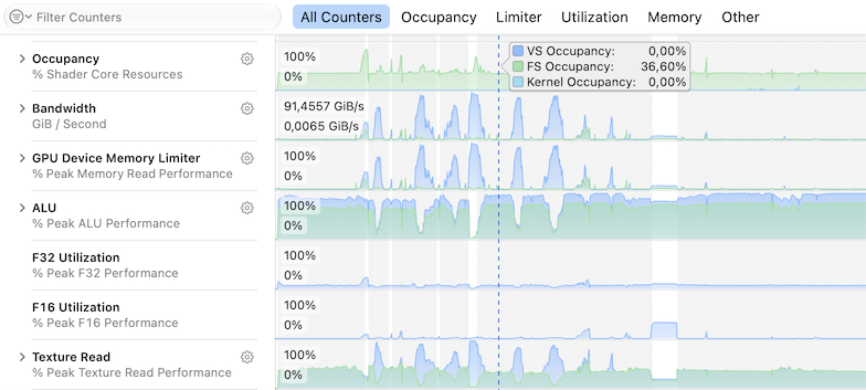
In particular, the shader’s occupancy is rather low:
- FS occupancy counter: 35.43 %
- Register allocation: 92
Before 2-level DDA, these numbers were:
- FS occupancy counter: 71.39 %
- Register allocation: 42
The DDA shader became a lot larger due to the nested loops. More state is being carried over the loop in registers. Here is a great post explaining why the occupancy (and register allocation) matters: https://interplayoflight.wordpress.com/2020/11/11/what-is-shader-occupancy-and-why-do-we-care-about-it/ In short, the GPU is able to schedule fewer groups of work on an execution unit concurrently, so memory stalls affect the performance negatively.
Reducing the size of the live state could bring the occupancy back up and improve the performance. But the ALU usage is also very high indicating that a lot of work is still being done despite the 2-level grid.
Fullscreen triangle
2026-07-27
Commit: dc0422d
Since per-pixel voxel ray tracing is expensive work, the fullscreen quad is replaced with a fullscreen triangle to avoid duplicated ray tracing along the quad edge. This is a good blog post explaining the method.
While it’s more optimal, there is no measurable difference at the granularity used here.
2-level DDA
2026-07-24
Commit: ed4004c
An additional brick grid is introduced, indicating whether an 8 x 8 x 8 group of voxels (a brick) is occupied. Like the voxel grid, the brick grid is a 3D texture:
|
|
And similarly, tracing the brick grid is identical to the voxel grid. However, when a brick is occupied, the brick is also traced using DDA:
|
|
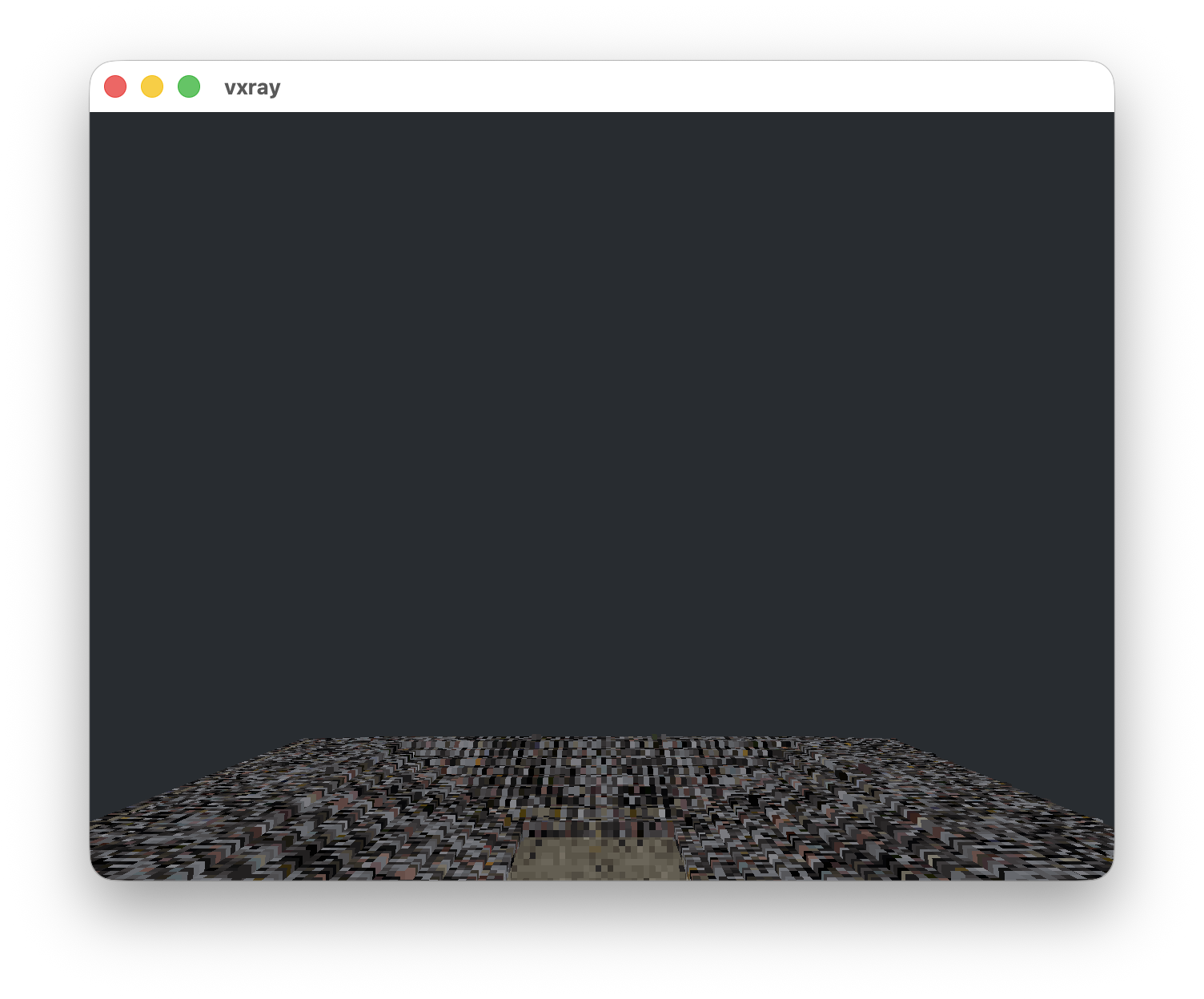
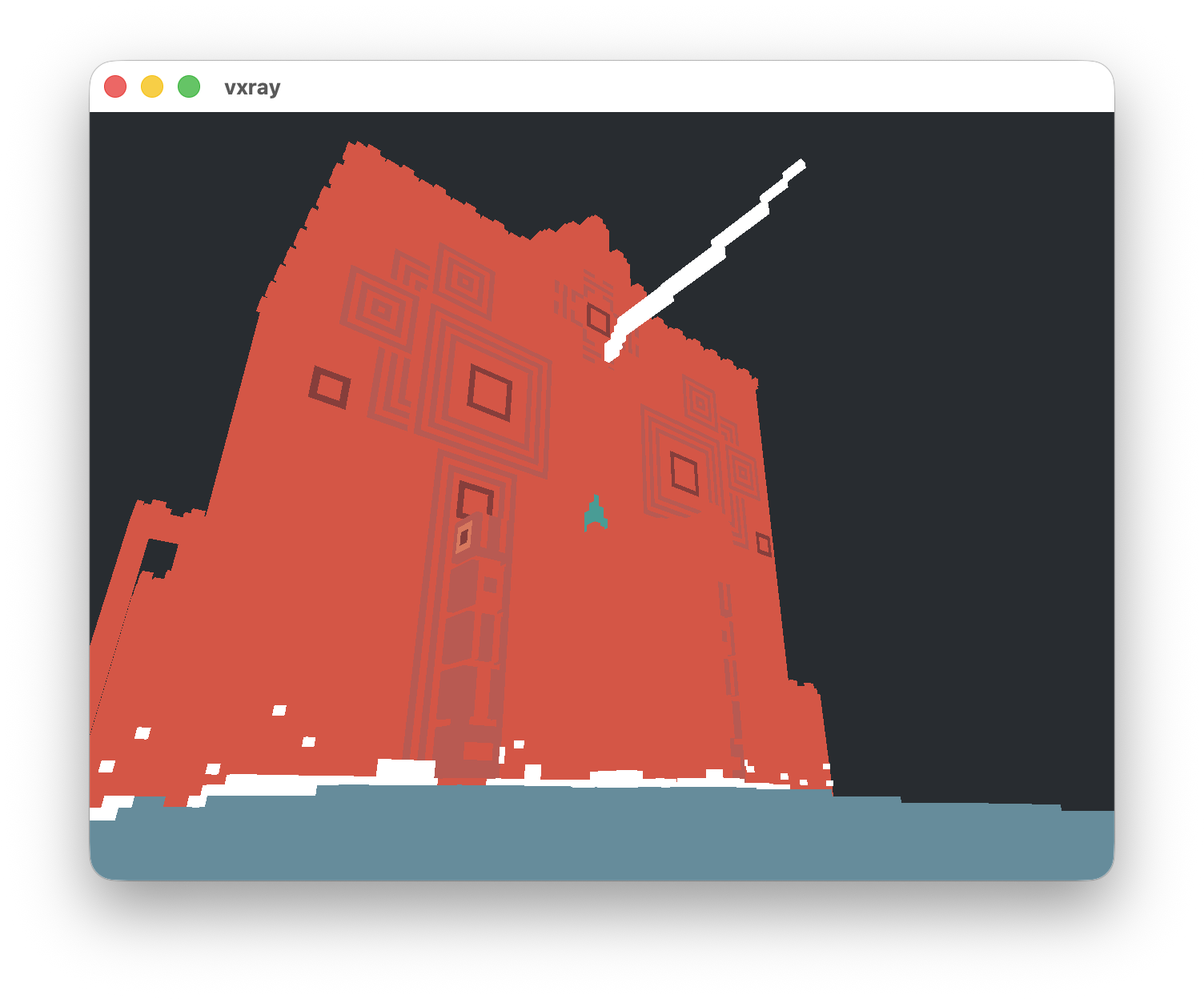
The FPS and average GPU walltime is measured at three locations on a Macbook Air (M2):
sponza-256-1
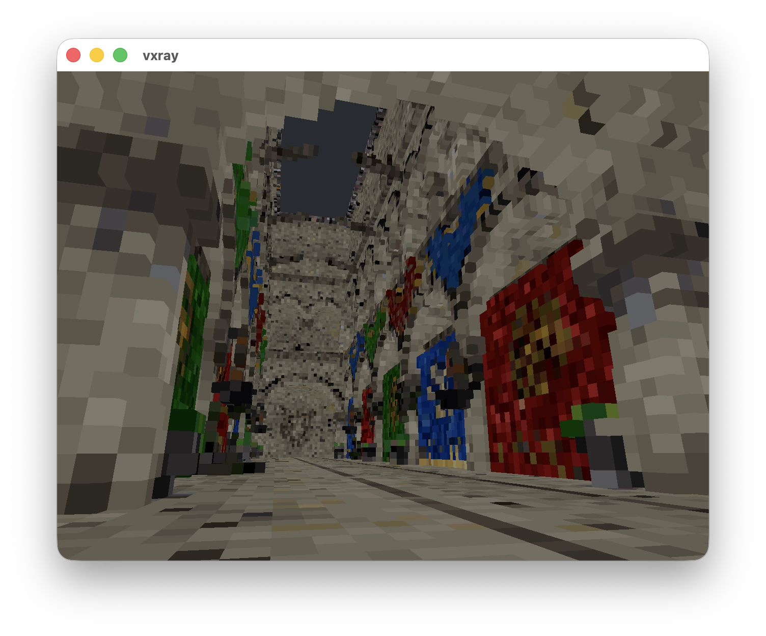
| Metric | Before | After | Uplift |
|---|---|---|---|
| FPS | 60.02 | 60.05 | +0.04% |
| Average GPU walltime | 14.80 ms | 14.63 ms | −1.16% |
sponza-256-2
| Metric | Before | After | Uplift |
|---|---|---|---|
| FPS | 21.07 | 60.04 | +184.93% |
| Average GPU walltime | 84.48 ms | 14.59 ms | −82.73% |
monu2-1
| Metric | Before | After | Uplift |
|---|---|---|---|
| FPS | 46.79 | 60.02 | +28.29% |
| Average GPU walltime | 32.50 ms | 14.23 ms | −56.21% |
Funnily enough, empty space was the heaviest to render before, as the kernel visited every single voxel along the ray before exiting.
With the brick grid in place, the rendering performance is now very steady, if not amazingly performant yet.
Camera presets
2026-07-22
Commit: f9e89c4
A simple camera preset file is introduced. Pressing F2 prints the current camera orientation as text:
|
|
Passing the text as a file to vxray spawns the camera at that position and orientation. This makes it easier to compare the performance at fixed locations with different models.
Voxelized test scenes
2026-07-21
This update does not contain changes in vxray.
Using my fork of voxquant, the Sponza Atrium mesh is voxelized into Mavigavoxel .vox files at different resolutions. A small modification is applied to the voxquant tool. Color palettes are padded up to 256 entries, in order to satisfy conservative Magicavoxel importers like the one I am using.
Here’s how I replaced the voxquant tool that I installed using cargo with my fork, cloned locally:
cargo install --path crates/voxquant --force
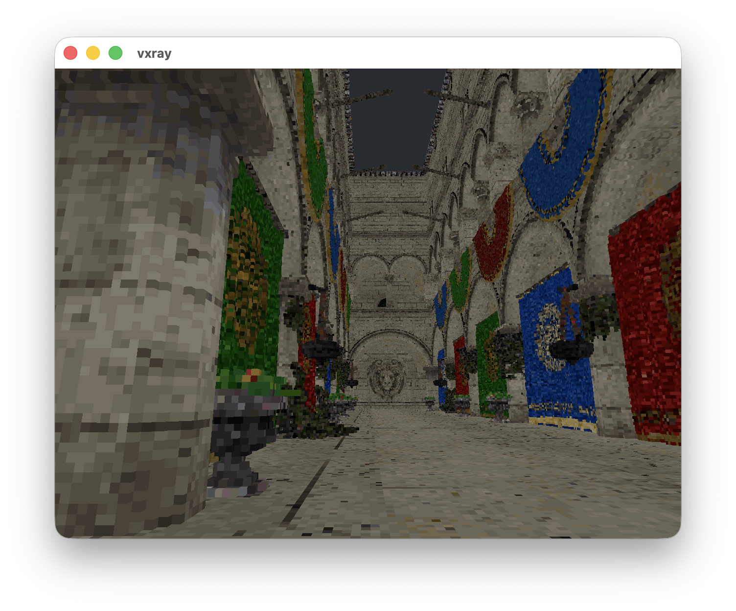
The Sponza Atrium scene at a 1024 grid resolution
3D voxel storage texture
2026-07-10
Commit: 67bf4a0
A 3D texture is used for storing the voxel grid.
|
|
Reading voxels from the texture is more straightforward than the byte buffer:
|
|
The voxels are laid out in memory as v = x + y * grid_extent + z * grid_extent². This makes it difficult to utilize the cache, as the ray tracing may have to access neighboring voxels grid_extent² apart from each other in memory. Using a 3D texture should help as it is designed for spatially adjacent data access.
The performance was measured again on a Macbook Air (M2).
| Metric | Before | After | Delta |
|---|---|---|---|
| FPS | 37.9 | 41.8 | 10.3% |
| Avg on-GPU | 41.94 ms | 35.99 ms | -14.2% |
Using a 3D texture results in less time spent on the GPU, although the improvement is not huge at this stage. A huge number of voxels are still being traversed by the algorithm.
Pack voxels into byte buffer
2026-07-08
Commit: 25b6fd2
Voxels are stored as bytes instead of wasteful uints:
|
|
Voxels are palette indices, with an index of 0 indicating empty space (hence, in Magicavoxel files, only palette indices > 0 are valid). The palette has 255 entries, so using a byte per voxel is sufficient.
Although peak memory consumption is reduced, there is no impact on runtime performance on a Macbook Air (M2):
| Metric | Before | After | Delta |
|---|---|---|---|
| FPS | 39.97 | 40.17 | +0.20 / +0.5% |
| On-GPU avg | 37.07 ms | 39.22 ms | +2.15 ms / 5.8% slower |
| Peak app memory | 115.80 MiB | 104.09 MiB | -11.70 MiB / -10.1% |
| Metal allocated size | 61.50 MiB | 61.50 MiB | 0.00 MiB |
Naive DDA
2026-07-04
Commit: 0014bd0
Render Magicavoxel models with naive DDA.
- Adds ogt_vox.h for parsing Magicavoxel files.
- Introduces DDA rendering in the pixel shader.
Here’s the gist of the DDA algorithm. For a ray with origin o and direction d, the point at t along the ray is given by
p = o + t * d
The first x-intersection is given by
t = (ceil(o.x) - o.x) / d.x
and similarly for the first y-intersection:
t = (ceil(o.y) - o.y) / d.y
Subsequent x and y-axis intersections are 1 unit apart: t = (ceil(o.x) - o.x) / d.x + (1 / d.x). The DDA algorithm keeps track of which intersection occurred first, and steps along the axis in that direction. The algorithm loops through the grid cells until a stopping condition is met, such as exiting the grid.
Here is a gist of the DDA algorithm, implemented in the pixel shader:
|
|
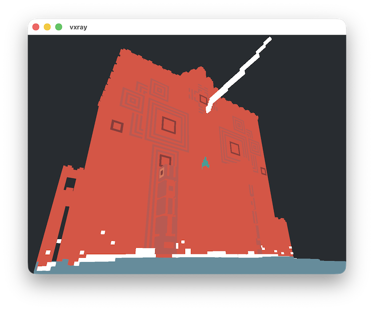
monu2.vox from ephtracy/voxel-model:
Hello, SDL!
2026-06-28
Commit: 03feb13
All projects have to start somewhere. The rendering infrastructure is set up to render a fullscreen quad.
- SDL_GPU is used as the rendering abstraction. The Metal backend is used on macOS, and the Vulkan backend on Windows.
- SDL_shadercross is used to compile/transpile HLSL shaders to SPIR-V and Metal.
- Shaders are compiled at build time and embedded as byte arrays into the source code.
A window opens displaying the UV coordinates as the color.