GPU Pathtracer Devlog

This post is a devlog for my rayfinder project. Follow along to see the progress, starting from scratch by opening a simple window.

First step towards temporal filtering: simple accumulation

2024-06-24

Commit: 29eebc8

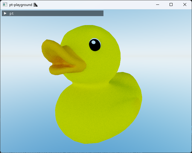
The first step towards temporal accumulation with a moving camera is implemented. The reference path tracer previously implemented temporal accumulation, but only when the camera was stationary. When the camera was moved, the render was invalidated and started from scratch.

The temporal accumulation is inspired by the Temporal AA and the Quest for the holy Trail blog post. The first two steps, jitter and resolve, are implemented here.

The jitter matrix offsets the image by a random subpixel amount each from, along the x and y axis. I used the 2-dimensional golden ratio sequence as a source of low-discrepancy values, just like previously in the animated blue noise section.

1
2
3
4

glm::mat4       jitterMat = glm::mat4(1.0f);
const glm::vec2 j = r2Sequence(frameCount, 1 << 20);
jitterMat[3][0] = (j.x - 0.5f) / framebufferSize.x;
jitterMat[3][1] = (j.y - 0.5f) / framebufferSize.y;

The view projection matrix is replaced with the view projection matrix multiplied by this jitter matrix. The image jitters slightly, yielding samples from different parts of the pixel over time.

Next, in the resolve pass, the pixel’s final color is computed based on the current and previous frame’s sample. The current color sample is computed in the lighting pass. The image no longer jitters after this accumulation step as the samples from the different parts of the pixel are averaged together to produce a stable pixel value.

 1
 2
 3
 4
 5
 6
 7
 8
 9
10
11
12
13
14

// The storage buffer populated by the raytracing compute shader.
@group(1) @binding(0) var<storage, read_write> sampleBuffer: array<array<f32, 3>>;
// The storage buffer for persisting the previous samples.
@group(1) @binding(1) var<storage, read_write> accumulationBuffer: array<array<f32, 3>>;

// elsewhere in code...

let sample = sampleBuffer[sampleBufferIdx];
let currentColor = vec3f(sample[0], sample[1], sample[2]);
let previousSample = accumulationBuffer[sampleBufferIdx];
let previousColor = vec3f(previousSample[0], previousSample[1], previousSample[2]);

color = 0.1 * currentColor + 0.9 * previousColor;
accumulationBuffer[sampleBufferIdx] = array<f32, 3>(color.r, color.g, color.b);

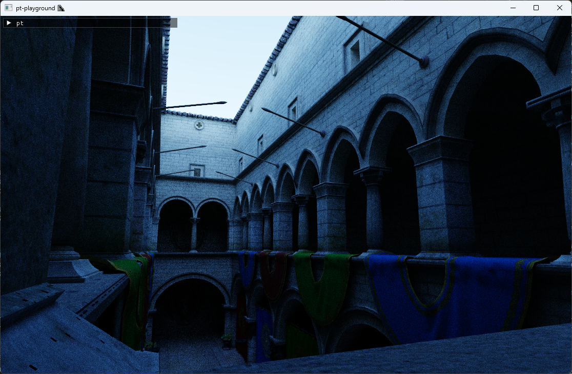
This simple sample accumulation produces an image with much less noise than before. However, the moving average alone does not account for the moving camera and results in ghosting artifacts due to camera motion.

Raytracing in a compute pipeline

2024-06-21

Commit: d06c8c9

Raytracing is moved from the fragment shader to a compute shader. The compute shader outputs the color into a storage buffer. A new render pass, the resolve pass, is introduced. It renders a fullscreen quad, and outputs the color from the storage buffer as the fragment color. The modification is fairly straightforward, except for one gotcha.

Previously, the depth buffer was sampled using a textureIdx calculated from the UV coordinate from the vertex shader.

1
2
3
4
5
6
7

let uv = in.texCoord;
let textureIdx = vec2u(floor(uv * uniforms.framebufferSize));
let depthSample = textureLoad(gbufferDepth, textureIdx, 0);

if depthSample == 0.0 {
    let world = worldFromUv(uv, depthSample);
// ...

The UV coordinate from the vertex shader is located at the center of the pixel, and is exactly where the depth sample is located.

In the compute shader, texture index and the UV coordinate is calculated the other way around. In the compute shader, we dispatch one job per pixel, and we can treat the global shader invocation id as a texture index. We compute the UV based on the texture index. This is the naive way of doing it:

1
2

let textureIdx = globalInvocationId.xy;
let uv = vec2f(globalInvocationId.xy) / uniforms.framebufferSize;

This will result in completely broken rendering (ask me how I know!).

The depth sample at textureIdx and the UV coordinate don’t align. The world space position we calculate from these two values is incorrect, resulting in ray self-intersection issues. The correct way to proceed is to place the UV coordinate at the center of the pixel, so that it matches the place where the depth sample was taken:

1
2

let textureIdx = globalInvocationId.xy;
let uv = (vec2f(globalInvocationId.xy) + vec2f(0.5)) / uniforms.framebufferSize;

With this in place, raytracing in the compute shader produces identical result to before.

Animated blue noise

2024-05-11

Commit: 18f5dbb

An improved sampling noise distribution is implemented.

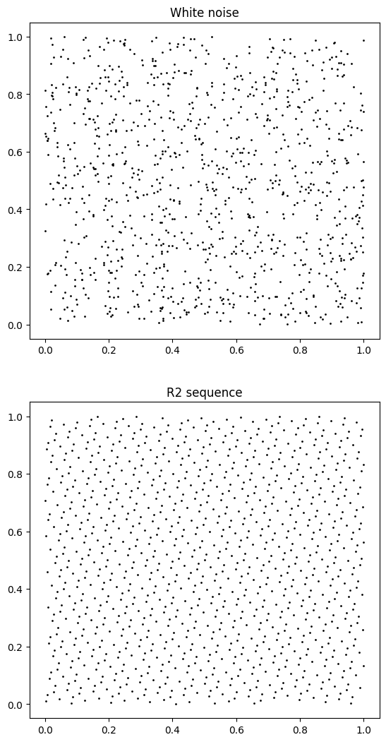
The type of noise used to produce the random numbers used to sample the light and surface normal has an impact on the final image. The pathtracer has been using “white noise” so far, so-called because it contains both high and low-frequency jitters. The randomly generated points can contain clusters and voids, and doesn’t necessarily cover the space very evenly.

Quasirandom numbers, such as the additive recurrence R-sequence (explained in depth in Unreasonable Effectiveness of Quasirandom Sequences), fill up the space much more evenly than regular random numbers (i.e. it has low spatial discrepancy):

R-sequences are very easy to generate. They are driven by a an increasing sequence of integers:

# See the "Unreasonable Effectiveness of Quasirandom Sequences" post for more definitions
def r2(n):
   g = 1.32471795724474602596
   a1 = 1.0/g
   a2 = 1.0/(g*g)
   return ((0.5+a1*n) % 1), ((0.5+a2*n) % 1)

The R-sequence can be used in place of white noise also when sampling random numbers in distributions or geometric primitives:

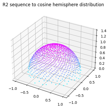
For each frame, you get a different value with very low spatial discrepancy. Unfortunately, the R2 sequence alone can’t be used to sample directions in the raytracing shader. Since each pixel has the same frame count, each pixel would be using the exact same sequence of “random numbers”. This results in visual artifacts, such as jittery shadows with bands.

Inspired by the article on Using Blue Noise for Ray Traced Soft Shadows, spatial decorrelation is added to the R2 sequence in the form of blue noise. Blue noise is explained in depth in the article, and is well worth a read. Unlike in the article, where a single channel of blue noise is used, and animated using a 1-dimensional R-sequence, I found it easier to work with two-dimensional blue noise and the R2 sequence. That way, I had no issues with the noise even over very large frame counts (n) for both soft shadows as well as sampling the cosine hemispheres.

To recap, the animated noise function has a spatial component (blue noise) and a temporal component (R2 sequence driven by the frame count).

 1
 2
 3
 4
 5
 6
 7
 8
 9
10
11
12
13
14
15
16

fn animatedBlueNoise(coord: vec2u, frameCount: u32, frameCountCycle: u32) -> vec2f {
    // Spatial component
    let idx = (coord.y % blueNoise.height) * blueNoise.width + (coord.x % blueNoise.width);
    let blueNoise = blueNoise.data[idx];

    // Temporal component
    let n = frameCount % frameCountCycle;
    let a1 = 0.7548776662466927f;
    let a2 = 0.5698402909980532f;
    let r2Seq = fract(vec2(
        a1 * f32(n),
        a2 * f32(n)
    ));

    return fract(blueNoise + r2Seq);
}

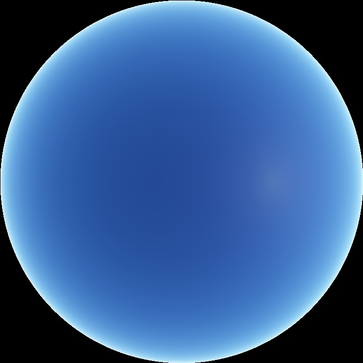
The source of blue noise values is a texture which can be downloaded from Free blue noise textures. Generating them yourself is tricky. Here’s an exmaple of a two-channel blue noise texture that I downloaded. The texture tiles seamlessly, so it can be used even when much smaller than the viewport.

The animated blue noise is then leveraged in all the places of the random number generator was previously used: generating the jittered primary ray origins, sampling directions in the cosine-weighted hemisphere, and sampling directions in the sun disk cone.

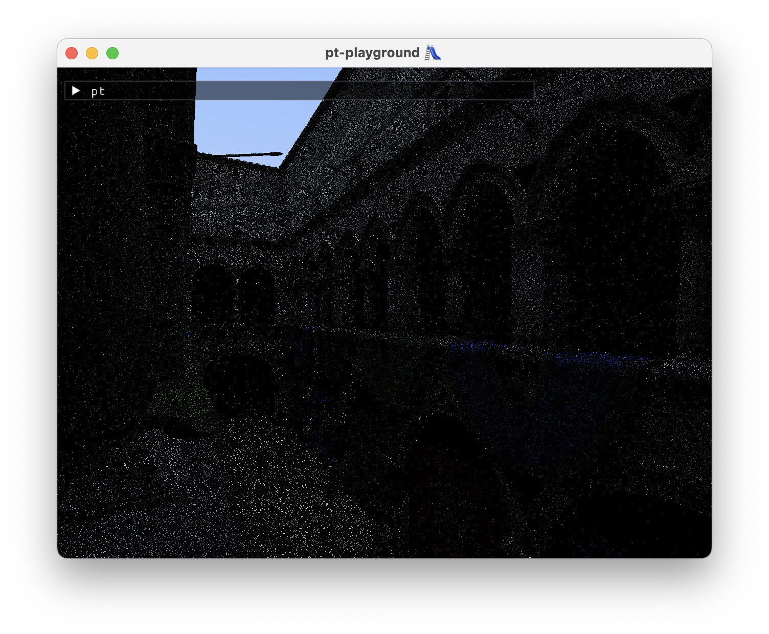
Here’s a comparison of the old white noise versus the new blue noise, at 1 sample per pixel.

White noise, 1 spp

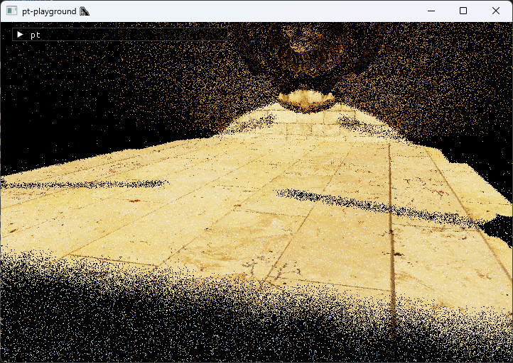
Blue noise, 1 spp

I hope the difference is apparent. I find the spatial distribution of blue noise to be much more pleasant.

At 16 samples per pixel, the difference is again noticeable.

White noise, 16 spp

Blue noise, 16 spp

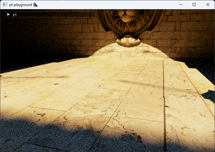
The animated blue noise results in much better soft shadows, and in slightly less noisy indirect illumination. Bounced light samples have so much variance that the blue noise has a reduced impact compared to soft shadows. But overall, using spatiotemporal blue noise significantly reduces the sample count required to obtain a clean image using the reference path tracer.

Deferred bounced lighting

2024-04-28

Commit: 7526265

Bounced lighting is added to the deferred render pipeline. The surfaceColor function now contains an identical diffuse sampling step as the reference path tracer. Output is identical to the reference path tracer without any accumulation.

 1
 2
 3
 4
 5
 6
 7
 8
 9
10
11
12
13
14
15
16
17
18
19
20
21
22
23
24
25
26
27
28
29
30
31
32
33
34
35
36
37
38
39
40
41
42
43
44

@must_use
 fn surfaceColor(rng: ptr<function, u32>, primaryPos: vec3f, primaryNormal: vec3f, primaryAlbedo: vec3f) -> vec3f {
     var position = primaryPos;
     var normal = primaryNormal;
     var albedo = primaryAlbedo;
     var radiance = vec3(0f);
     var throughput = vec3(1f);

     radiance += throughput * lightSample(rng, position, normal, albedo);

     for (var bounce = 1; bounce < NUM_BOUNCES; bounce += 1) {
         let wi = evalImplicitLambertian(normal, rng);
         let ray = Ray(position, wi);
         throughput *= albedo;

         var hit: Intersection;
         if rayIntersectBvh(ray, T_MAX, &hit) {
             position = hit.p;
             normal = hit.n;
             let uv = hit.uv;
             let textureDescriptorIdx = hit.textureDescriptorIdx;
             albedo = evalTexture(textureDescriptorIdx, uv);
         } else {
             let v = ray.direction;
             let s = skyState.sunDirection;

             let theta = acos(v.y);
             let gamma = acos(clamp(dot(v, s), -1f, 1f));

             let skyRadiance = vec3f(
                 skyRadiance(theta, gamma, CHANNEL_R),
                 skyRadiance(theta, gamma, CHANNEL_G),
                 skyRadiance(theta, gamma, CHANNEL_B)
             );

             radiance += throughput * skyRadiance;
             break;
         }

         radiance += throughput * lightSample(rng, position, normal, albedo);
     }

     return radiance;
 }

Support for larger scenes

2024-04-27

Commit: 26030ac

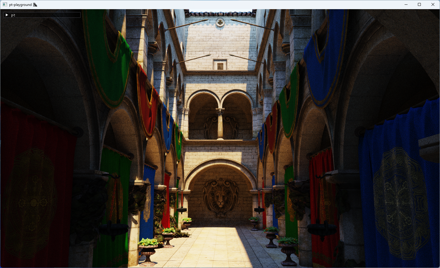
A number of changes have been made over the last few weeks to support the loading and rendering of additional, larger, scenes.

• Make positionOffset more conservative to help with larger scenes. In order to fight some remaining z-fighting which occurs in the distance of large open spaces, the position offset from the intersected geometry is made more conservative than before.
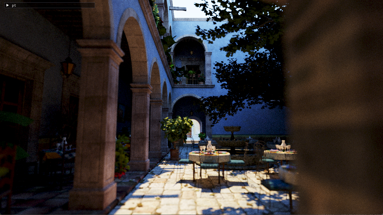
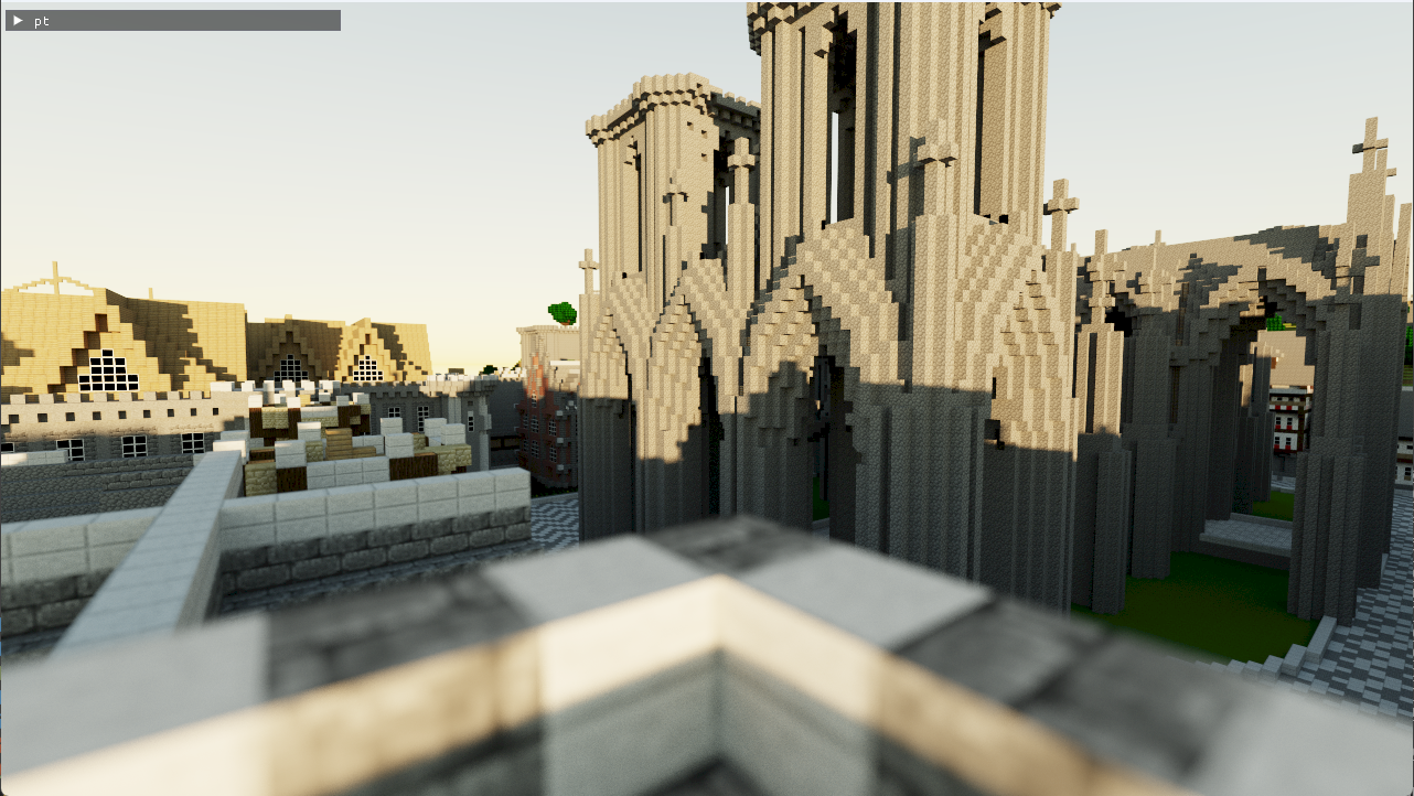
• Load single pixel textures. The San Miguel courtyard scene contains single pixel textures, stored in the "baseColorFactor" field in glTF.
• Increase GPU limits to unconstrain size of resources that can be used. The San Miguel and Rungholt minecraft scene both contain close to a gigabyte of geometry and textures. The GPU adapter limits are increased to accommodate the new scene sizes.
  • Related: Throw exception when gpu buffer fails to map on creation. Improved error reporting when a memory map request occurs over the device buffer size limit.
• Bump dawn to chromium/6385. The latest version of Dawn fixes some Vulkan allocator OOM errors which occur when creating buffers within the new, larger, device limits.

New scenes: rayfinder-assets.

san-miguel-low-poly.glb

rungholt.glb

Deferred direct lighting

2024-04-22

Commit: 2f59399

Direct lighting is added to the lighting pass. The primary ray intersection with the scene is reconstructed from the gbuffers using a slightly modified version of the function from the previous entry.

1
2
3
4
5
6

fn worldFromUv(uv: vec2f, depthSample: f32) -> vec3f {
    let ndc = vec4(2.0 * vec2(uv.x, 1.0 - uv.y) - vec2(1.0), depthSample, 1.0);
    let worldInvW = uniforms.inverseViewReverseZProjectionMat * ndc;
    let world = worldInvW / worldInvW.w;
    return world.xyz;
}

The surface normal and the albedo are looked up as-is from their respective buffers.

The direct lighting contribution for each pixel is obtained by tracing a ray to the sun disk and testing for visibility. This snippet is identical to the direct lighting contribution from the “next event estimation” contribution in the reference path tracer.

 1
 2
 3
 4
 5
 6
 7
 8
 9
10
11
12
13

fn surfaceColor(rng: ptr<function, u32>, pos: vec3f, normal: vec3f, albedo: vec3f) -> vec3f {
    let lightDirection = sampleSolarDiskDirection(
        SOLAR_COS_THETA_MAX, skyState.sunDirection, rng);
    let lightIntensity = vec3(
        skyState.solarRadiances[CHANNEL_R],
        skyState.solarRadiances[CHANNEL_G],
        skyState.solarRadiances[CHANNEL_B]
    );
    let brdf = albedo * FRAC_1_PI;
    let reflectance = brdf * dot(normal, lightDirection);
    let lightVisibility = shadowRay(Ray(pos, lightDirection), T_MAX);
    return lightIntensity * reflectance * lightVisibility * SOLAR_INV_PDF;
}

This results in the following image with harsh, direct, sun light. Indirect light or sky dome light is not visible since no bounce rays are being traced yet.

Solving z-fighting issues with the depth buffer

The direct lighting didn’t work completely out of the box. Very visible z-fighting occurred, presumably the sun visibility ray self-intersecting with the scene geometry due to the world space coordinate calculated from the depth buffer lacking precision.

The Depth Precision Visualized is a great visual explanation of depth buffer precision problems.

There were two ways to solve the problem:

1. Choosing a larger near plane value to reduce the steepness of the \(1/z\) asymptote.
2. Reversing the near and far plane, i.e. reverse Z projection.

Moving the near plane a bit further away from zero (from 0.1 to > 0.5) actually solved the z-fighting issue, but also caused visible clipping when moving around the Sponza scene.

Reverse Z projection is implemented, in the three steps mentiond in this blog post (depth comparison function to greater instead of less, clear the depth buffer with 0 instead of 1, and multiply the projection matrix with the reverse-z matrix to flip the planes).

 1
 2
 3
 4
 5
 6
 7
 8
 9
10
11
12
13
14
15
16
17
18

glm::mat4 FlyCameraController::viewReverseZProjectionMatrix() const
{
    // ...

    const glm::mat4 reverseZ = glm::mat4(1.0f, 0.0f,  0.0f, 0.0f,
                                         0.0f, 1.0f,  0.0f, 0.0f,
                                         0.0f, 0.0f, -1.0f, 0.0f,
                                         0.0f, 0.0f,  1.0f, 1.0f);

    const float     near = 0.1f;
    const float     far = 1000.0f;
    const glm::mat4 project =
        glm::perspective(mVfov.asRadians(), aspectRatio(mWindowSize), near, far);

    const glm::mat4 view = glm::lookAt(origin, lookAt, up);

    return reverseZ * project * view;
}

Rendering the sky and albedo in a deferred render pass

2024-03-31

Commit: 41ee498

The HybridRenderer is renamed DeferredRenderer as that is a more frequently used term in this log and literature.

A new deferred lighting pass is introduced. The sky and gbuffer’s albedo channel is rendered as a proof of concept.

The shader renders a full-screen quad to the screen and uses the screen’s UV-coordinates to calculate the pixel’s camera ray direction as well as the texture index to read a pixel from the albedo texture. The depth buffer value is used to test whether the pixel overlaps geometry or the sky. The sentinel value of 1.0 is what the depth buffer was cleared with and indicates that the pixel did not contain geometry.

 1
 2
 3
 4
 5
 6
 7
 8
 9
10
11
12
13
14
15
16
17
18
19
20
21
22

// fragment shader body
var color = vec3f(0.0, 0.0, 0.0);

let uv = in.texCoord;
let idx = vec2u(floor(uv * uniforms.framebufferSize));
let d = textureLoad(gbufferDepth, idx, 0);
if d == 1.0 {
    let world = worldFromUv(uv);
    let v = normalize((world - uniforms.cameraEye).xyz);
    let s = skyState.sunDirection;
    // This is equivalent to path tracer code
    let theta = acos(v.y);
    let gamma = acos(clamp(dot(v, s), -1f, 1f));
    color = vec3f(
        skyRadiance(theta, gamma, CHANNEL_R),
        skyRadiance(theta, gamma, CHANNEL_G),
        skyRadiance(theta, gamma, CHANNEL_B)
    );
} else {
    let albedo = textureLoad(gbufferAlbedo, idx, 0).rgb;
    color = albedo;
}

The function worldFromUv uses the inverse view projection matrix to calculate near projection plane coordinates from the given UV coordinate. The UV coordinate can be transformed into a normalized device coordinate \(\mathbf{x}_{ndc}\) on the camera frustum’s near plane, but it will be scaled by \(1 / w\) value from the divide-by-w step:

$$ \begin{bmatrix} {x} / {w_0} \\ {y} / {w_0} \\ {z} / {w_0} \\ {1} / {w_0} \end{bmatrix} = (\mathrm{PV})^{-1} \mathbf{x}_{ndc} $$

We need to divide all values by the vector’s w component to obtain the original coordinates before the divide-by-w step.

1
2
3
4
5
6

fn worldFromUv(uv: vec2f) -> vec4f {
    let ndc = vec4(2.0 * vec2(uv.x, 1.0 - uv.y) - vec2(1.0), 0.0, 1.0);
    let worldInvW = uniforms.inverseViewProjectionMat * ndc;
    let world = worldInvW / worldInvW.w;
    return world;
}

The lighting pass displays just the albedo and looks a bit dull at the moment.

The path traced result for reference. Note that the sky is exactly the same is in the deferred pass.

First steps towards a deferred renderer 👣

2024-03-30

Commit: 3d1c871

A new deferred renderer, the HybridRenderer class, is added alongside the existing path tracer. The deferred renderer will use path tracing for lighting, but it will replace the primary ray-scene intersection with the output of the rasterization pipeline, which is much faster than using a ray tracing.

As of now, the renderer uses the rasterization pipeline to render the geometry into the gbuffer textures. The albedo and normal textures are render attachments of the gbuffer render pass. The position doesn’t have it’s own distinct texture. Instead, the depth buffer can be reused to calculate the world positions of each pixel.

 1
 2
 3
 4
 5
 6
 7
 8
 9
10

struct GbufferOutput {
    @location(0) albedo: vec4<f32>,
    @location(1) normal: vec4<f32>,
}

@fragment
fn fsMain(in: VertexOutput) -> GbufferOutput {
    var c = pow(textureSample(texture, textureSampler, in.texCoord).xyz, vec3(2.2f));
    return GbufferOutput(vec4(c, 1f), vec4(normalize(in.normal.xyz), 1f));
}

The locations of the GbufferOutput map to the color attachments array:

 1
 2
 3
 4
 5
 6
 7
 8
 9
10
11
12
13
14
15
16
17
18
19

const std::array<WGPURenderPassColorAttachment, 2> colorAttachments{
            WGPURenderPassColorAttachment{
                .nextInChain = nullptr,
                .view = albedoTextureView,
                .depthSlice = WGPU_DEPTH_SLICE_UNDEFINED,
                .resolveTarget = nullptr,
                .loadOp = WGPULoadOp_Clear,
                .storeOp = WGPUStoreOp_Store,
                .clearValue = WGPUColor{0.0, 0.0, 0.0, 1.0},
            },
            WGPURenderPassColorAttachment{
                .nextInChain = nullptr,
                .view = normalTextureView,
                .depthSlice = WGPU_DEPTH_SLICE_UNDEFINED,
                .resolveTarget = nullptr,
                .loadOp = WGPULoadOp_Clear,
                .storeOp = WGPUStoreOp_Store,
                .clearValue = WGPUColor{0.0, 0.0, 0.0, 1.0},
            }};

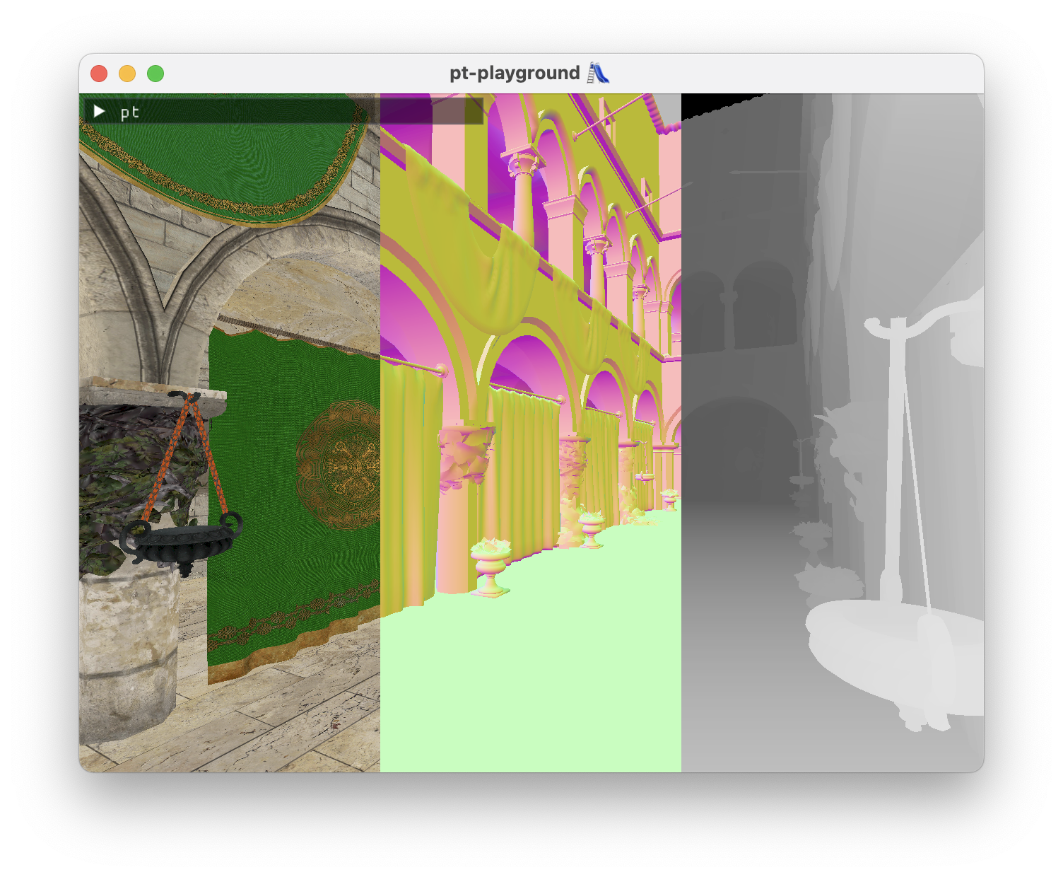
A debug renderer is also added which shows the three buffers side by side. The depth buffer is displayed without actually transforming the coordinates back to world space – at this stage it’s possible to visually assert that the textures are being bound correctly to the shader.

Gallery of failures

2024-03-29

A small break from the usual progress entries. Instead, two images from unsuccesful attempts to render a 3d model using the regular rasterization pipeline.

Umm, was I supposed to use an index buffer to access the vertices?

The model textures are BGRA8Unorm, not RGBA8Unorm, aren’t they?

Copying shader source files into a string at build time

2024-03-22

Commit: a5207ab

A method for copying WGSL shader source automatically into a C-string is implemented. The shader source files are listed in the main CMakeLists.txt:

1
2
3
4
5

set(WGSL_SHADER_FILES
    reference_path_tracer.wgsl
    texture_blit.wgsl
    hybrid_renderer_gbuffer_pass.wgsl
    hybrid_renderer_debug_pass.wgsl)

The custom target bake-wgsl copies each source file’s content into a string in the pt/shader_source.hpp header file. The main pt target depends on the bake-wgsl target so that every time a build occurs, shader_source.hpp is updated. This makes it possible to edit shaders in separate source files with the benefits of the wgsl-analyzer plugin.

The custom target depends on a custom command which outputs the header file. The custom command is implemented as a separate cmake script, so that it can be called from the custom command.

1
2
3
4
5
6
7
8

include(cmake/BakeWgslSource.cmake)
add_custom_command(
    OUTPUT ${SHADER_SOURCE_HEADER_FILE}
    COMMAND ${CMAKE_COMMAND} -DCALL_BAKE_WGSL_SOURCE=1 -DOUTPUT_FILE=${SHADER_SOURCE_HEADER_FILE} -DWGSL_FILES="${WGSL_SHADER_FILES}" -P ${CMAKE_SOURCE_DIR}/cmake/BakeWgslSource.cmake
    COMMENT "Generating ${SHADER_SOURCE_HEADER_FILE} from .wgsl files"
    WORKING_DIRECTORY ${CMAKE_SOURCE_DIR}
)
add_custom_target(bake-wgsl DEPENDS ${SHADER_SOURCE_HEADER_FILE})

Depth of field using the thin lens approximation

2024-01-14

Commit: 0b77f54

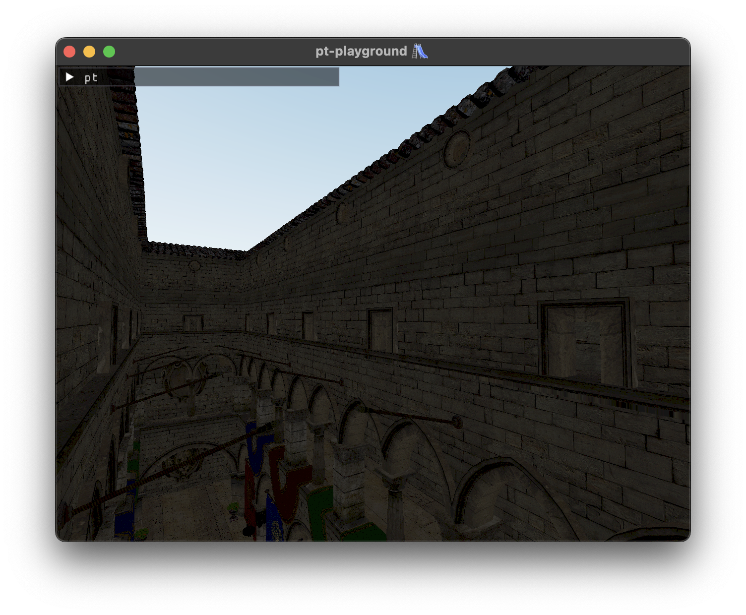
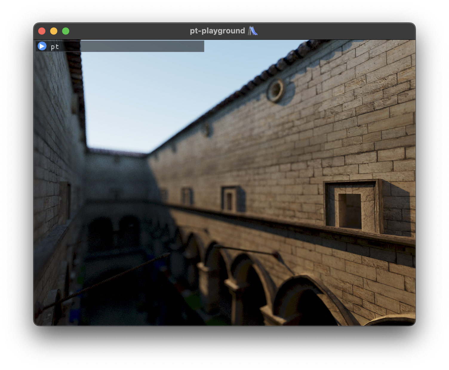
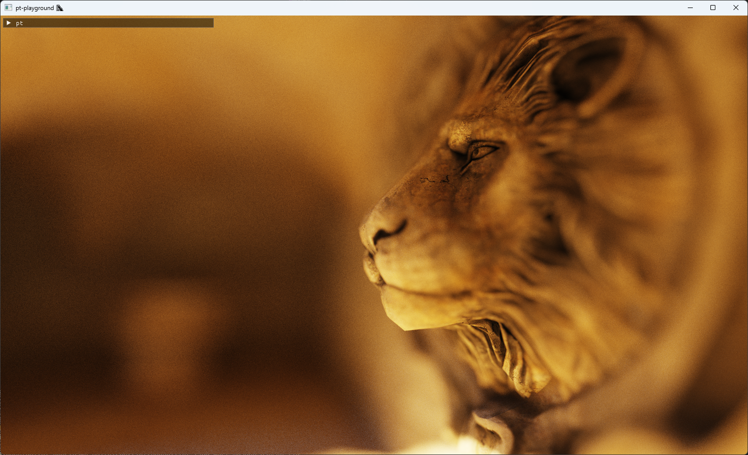
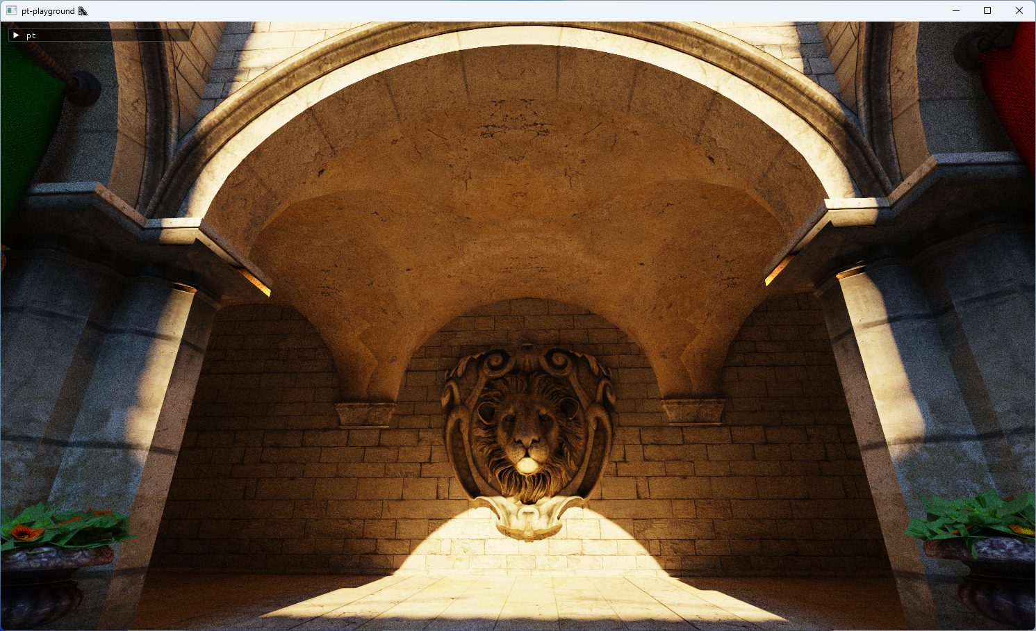
The thin lens approximation is implemented. The thin lens approximation models a simple lens with an aperture, allowing generating convincing looking depth of field effects.

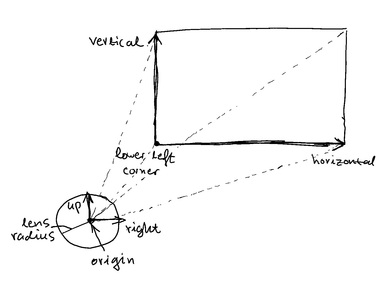
The thin lens approximation uses the following coordinate system. Normally, rays are generated at origin, and point at each pixel on the image plane (the plane with lower left corner). Using the thin lens approximation, rays are generated randomly in a disk about origin with a lens radius. This approximates the behavior of a ray of light passing through a lens aperture through the focal point, just reversed from a real lens; the focal point is in front of the lens, instead of behind it.

This is how ray generation works in the shader:

 1
 2
 3
 4
 5
 6
 7
 8
 9
10
11
12

fn generateCameraRay(camera: Camera, rngState: ptr<function, u32>, u: f32, v: f32) -> Ray {
    let randomPointInLens = camera.lensRadius * rngNextVec2InUnitDisk(rngState);
    let lensOffset = randomPointInLens.x * camera.right + randomPointInLens.y * camera.up;

    let origin = camera.origin + lensOffset;
    let direction = normalize(camera.lowerLeftCorner
                              + u * camera.horizontal
                              + v * camera.vertical
                              - origin);

    return Ray(origin, direction);
}

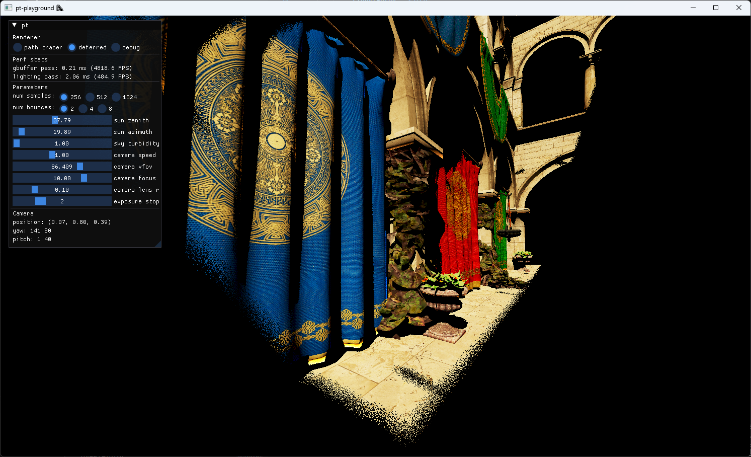
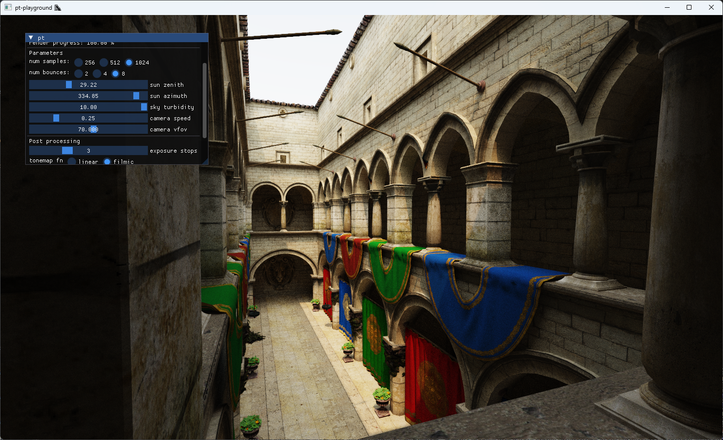
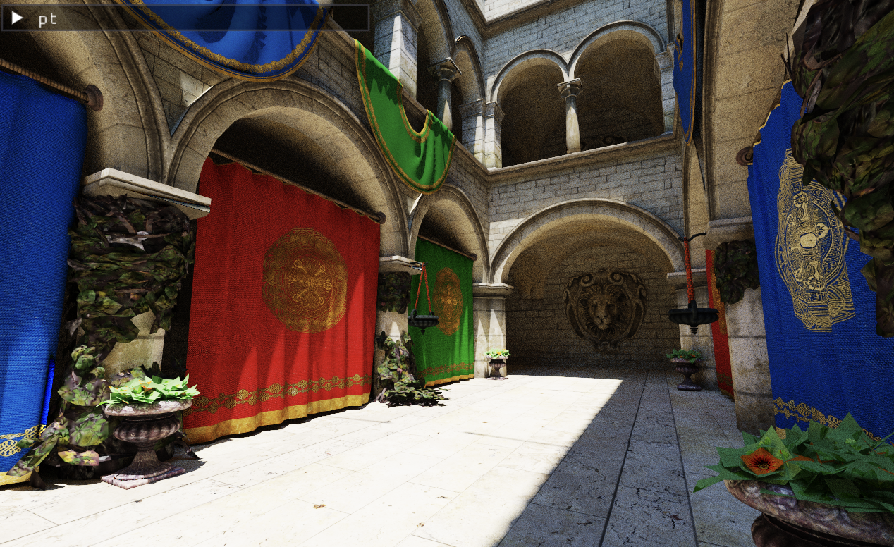
UI controls are added which allow the selection of the lens radius, as well as the focus distance. In order to get accurate focus on e.g. the lion’s eye, “click to focus” is also implemented, which calculates the focus distance to the point under the mouse cursor. This is implemented by retaining the BVH in the CPU program, and doing a ray-BVH intersection test by generating a ray at the mouse coordinates.

Adding atmospheric turbidity controls

2024-01-07

Commit: e0fe5f4

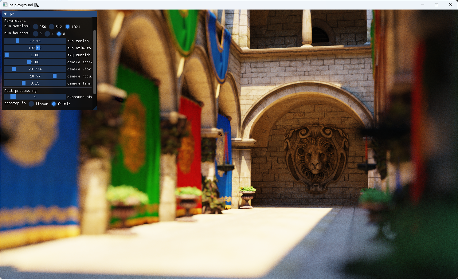
The updated sky model interpolates between the different sky and solar radiances at different atmospheric turbidities. A UI control is added to allow the selection of different turbidity values to see their effect on the image.

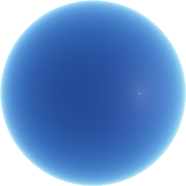
A turbidity of 1 corresponds to a very clear sky. The sun is very bright compared to the sky dome. With a turbidity of 10, a large quantity of light from the sun of all wavelengths is scattered. The sky is less blue as a result, and the sunlight’s intensity is much smaller. The effect looks a bit like an overcast day.

Turbidity 1:

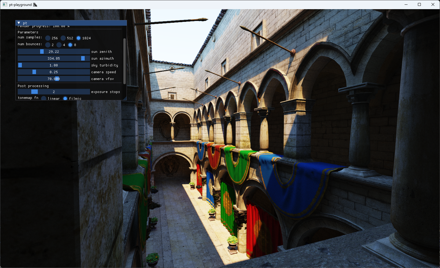
Turbidity 7:

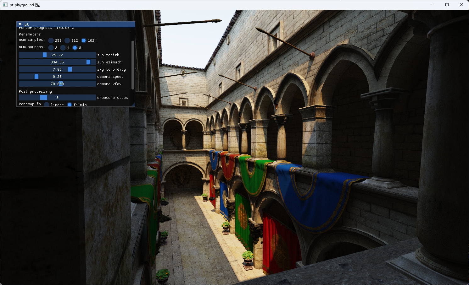
Turbidity 10:

Adding physically-motivated sunlight to the scene ☀️

2024-01-01

Commit: 7f69e97

Physically-motivated sun disk radiance is added to the scene.

The original sample code from the Sky Dome Appearance Project is added to the pathtracer project. The sky dome model contains a code path for calculating sunlight. The model provides spectral radiance across the sun disk.

In order to incorporate the sun into the pathtracer, the sun disk spectral radiances need to be converted to RGB values. Spectral radiance \(L\) can be converted to CIE XYZ values using integrals with published color matching functions (CMFs):

$$ X = \int_{\lambda} L(\lambda)\bar{x}(\lambda) d \lambda $$ $$ Y = \int_{\lambda} L(\lambda)\bar{y}(\lambda) d \lambda $$ $$ Z = \int_{\lambda} L(\lambda)\bar{z}(\lambda) d \lambda $$

The following image illustrates the integration of the spectral radiances with the CMFs for the XYZ color space:

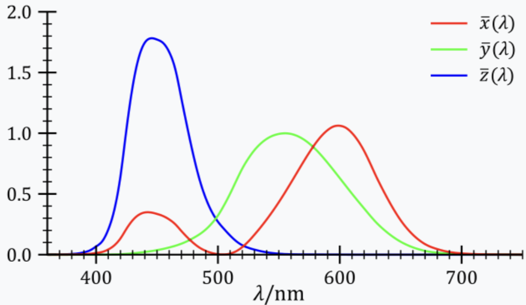
C code from the Simple Analytic Approximations to the CIE XYZ Color Matching Functions paper was used to implement simple multi-lobe Gaussian fits for the CIE XYZ CMFs.

The sky dome model is used to generate solar radiances across the entire sun disk at 10 different turbidities. The spectral radiance and CMF product is integrated using the trapezoidal method for each XYZ component.

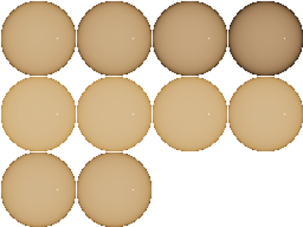
Technical note: the sun disks contain a bright spot, which I didn’t spend time on figuring out yet. The model implementation appears to be a bit incomplete and therefore some issues might remain. Since averages are computed across the sun disk anyway, the bright spot does not affect the computed radiance very much.

For each turbidity, the solar radiance is converted to XYZ, then to sRGB primaries. The XYZ to sRGB conversion matrix was obtained here. The mean of the sRGB primaries is computed and used as a proxy of the solar radiance over the sun disk. The hw-skymodel library interpolates between these mean RGB solar radiances to account for the different solar intensities at different atmospheric turbidities.

The solar radiance can now be generated along with the sky dome radiance.

The earlier, hard-coded lightIntensity value is now replaced with the computed mean RGB solar radiance.

1
2
3
4
5

let lightIntensity = vec3(
    skyState.solarRadiances[CHANNEL_R],
    skyState.solarRadiances[CHANNEL_G],
    skyState.solarRadiances[CHANNEL_B]
);

This results in a more beautiful yellowish lighting in the scene.

Technical note: in the actual pathtracer shader, the sky dome radiance code path skips the sun disk radiance. This means that the sun disk is not visible in the sky in images produced by the pathtracer. Including the sun disk radiance when the ray scatters into the sky results in images with fireflies. This is likely due to some very rare rays which eventually hit the sun disk directly with large weights.

Quick color encoding fix

2023-12-30

Commit: 883ed07

Two issues with color encoding are fixed.

• Textures stored in image files typically contain a standard non-linear gamma ramp, and need to be converted to linear values during sampling. Non-linear RGB values cannot be mutually added or multiplied, so the color calculations have not been correct up until now.
• The frame buffer’s texture format is WGPUTextureFormat_BGRA8Unorm and a gamma ramp must be applied to the final image output colors.

The duck without the sun – the image appears less washed out than before.

The difference in the Sponza scene is less pronounced, but the shadows seem to be a bit brighter than before.

Adding sunlight to the scene

2023-12-28

Commit: 70624a7

Previously, the Sponza scene has appeared rather dimly lit. The sky dome acts like a giant diffuse light source, since the sky dome model used does not actually contain a sun disk, the main light source.

The sun disk’s angular radius is 0.255 degrees, which means that it occupies so little space in the sky that few rays would actually hit it with random chance. The “Next Event Estimation” method is implemented to sample the sun efficiently. The method samples the sun disk on every ray-triangle intersection and evaluates the material’s BRDF to accumulate the sun’s radiance at every ray bounce. The sun’s direct illumination is used as indirect illumination in the following bounces.

 1
 2
 3
 4
 5
 6
 7
 8
 9
10
11
12
13
14
15
16
17
18

loop {
    var hit: Intersection;
    if rayIntersectBvh(ray, T_MAX, &hit) {
        let albedo = evalTexture(hit.textureDescriptorIdx, hit.uv);
        let p = hit.p;

        // Sample a random direction towards the sun disk.
        let lightDirection = sampleSolarDiskDirection(
                SOLAR_COS_THETA_MAX, skyState.sunDirection, rngState);
        // Hard-coded sun radiance with plausible magnitude.
        let lightIntensity = vec3f(1000000f, 1000000f, 1000000f);
        let brdf = albedo * FRAC_1_PI;
        let reflectance = brdf * dot(hit.n, lightDirection);
        let lightVisibility = shadowRay(Ray(p, lightDirection), T_MAX);
        radiance += throughput * lightIntensity * reflectance *
                    lightVisibility * SOLAR_INV_PDF;

    // The rest of the rendering loop as before

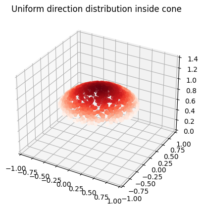
sampleSolarDiskDirection is based on the sampling transformation function presented in Sampling Transformations Zoo, Ray Tracing Gems. It generates random directions in a cone, subtended by a disk with an angular radius, \(\theta_{\mathrm{max}}\). The directions have to be transformed into the sun’s direction, using the pixarOnb orthonormal basis function.

 1
 2
 3
 4
 5
 6
 7
 8
 9
10
11
12
13
14

fn rngNextInCone(state: ptr<function, u32>, cosThetaMax: f32) -> vec3f {
    let u1 = rngNextFloat(state);
    let u2 = rngNextFloat(state);

    let cosTheta = 1f - u1 * (1f - cosThetaMax);
    let sinTheta = sqrt(1f - cosTheta * cosTheta);
    let phi = 2f * PI * u2;

    let x = cos(phi) * sinTheta;
    let y = sin(phi) * sinTheta;
    let z = cosTheta;

    return vec3(x, y, z);
}

The value of lightIntensity is a very large value, with a roughly plausible order of magnitude, which results in a good looking image. In the future it could be derived from a physically based model of the sun.

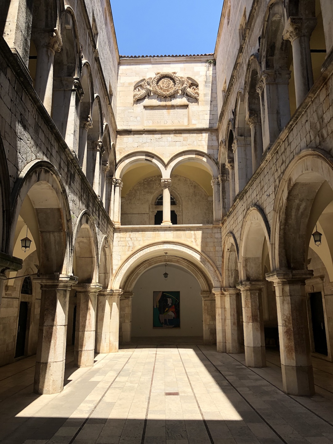
Finally, here’s a picture of what the Sponza palace looks like in real life, from a picture that I took when I visited there in 2022.

Implementing tiled texture support

2023-12-24

Commit: e190c51

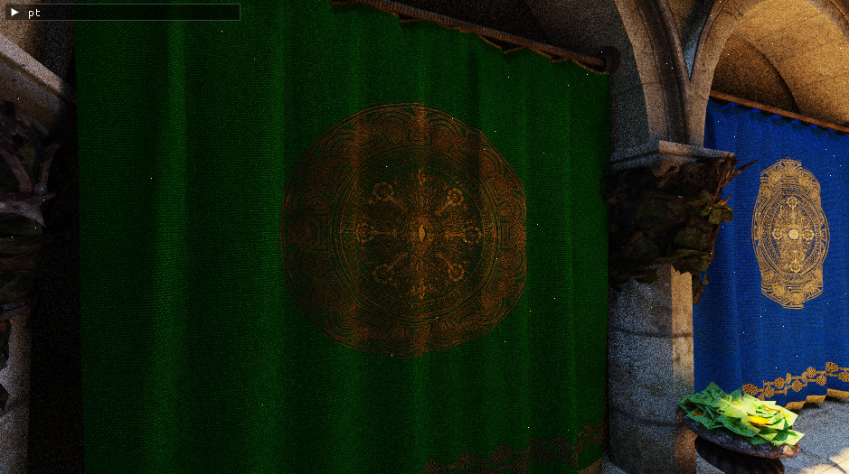
In the Simple texture support section, an apparent texture issue with the Sponza atrium scene was highlighted. On further investigation, the 3d model’s texture coordinates were not contained in the [0, 1] range, which is what my texture sampler assumes. To look correct, the model assumes tiled texture coordinate support in the renderer. The texture coordinate is supposed to wrap around back to zero at a regular interval.

The issue can be clearly seen in the corners of the model where the texture is displayed correctly once, and then gets stretched out as the texture coordinate fails to wrap around.

In glTF, by default, textures are assumed to be sampled using OpenGL’s GL_REPEAT behavior. This can be confirmed by observing cgltf_texture::sampler::wrap_s and wrap_t values:

1
2
3
4
5

// Look up OpenGL texture wrap mode magic numbers:
// https://registry.khronos.org/OpenGL/api/GL/glcorearb.h
// GL_REPEAT: 10497
assert(baseColorTexture.sampler->wrap_s == 10497);
assert(baseColorTexture.sampler->wrap_t == 10497);

The OpenGL spec says that

• GL_REPEAT causes the integer part of the s coordinate to be ignored; the GL uses only the fractional part, thereby creating a repeating pattern.

To mimic GL_REPEAT behavior, the UV coordinates are passed through the fract function during texture lookup:

1
2
3
4
5

fn textureLookup(desc: TextureDescriptor, uv: vec2f) -> vec3f {
    let u = fract(uv.x);
    let v = fract(uv.y);

    // .. the rest of the function as before

With this simple change, the Sponza scene looks correct and it finally feels right to give it the path tracer treatment.

Avoiding triangle self-intersection

2023-12-17

Commit: 9183d42

It’s possible for the ray-triangle intersection point to be below the triangle if one isn’t careful, resulting in the next ray self-intersecting the triangle. The method from A Fast and Robust Method for Avoiding Self-Intersection, Ray Tracing Gems is implemented. It contains two parts.

First, the intersection point should be computed using barycentric coordinates, instead of the ray equation, to avoid precision issues due to the difference in magnitude of the ray origin and the distance.

Second, the intersection point is offset from the surface of the triangle using the following offsetRay function. It offsets using a conservative estimate of the precision error, accounting for the scale of the intersection point.

 1
 2
 3
 4
 5
 6
 7
 8
 9
10
11
12
13
14
15
16
17
18
19

const ORIGIN = 1f / 32f;
const FLOAT_SCALE = 1f / 65536f;
const INT_SCALE = 256f;

fn offsetRay(p: vec3f, n: vec3f) -> vec3f {
    let offset = vec3i(i32(INT_SCALE * n.x), i32(INT_SCALE * n.y), i32(INT_SCALE * n.z));
    // Offset added straight into the mantissa bits to ensure the offset is scale-invariant,
    // except for when close to the origin, where we use FLOAT_SCALE as a small epsilon.
    let po = vec3f(
        bitcast<f32>(bitcast<i32>(p.x) + select(offset.x, -offset.x, (p.x < 0))),
        bitcast<f32>(bitcast<i32>(p.y) + select(offset.y, -offset.y, (p.y < 0))),
        bitcast<f32>(bitcast<i32>(p.z) + select(offset.z, -offset.z, (p.z < 0)))
    );

    return vec3f(
        select(po.x, p.x + FLOAT_SCALE * n.x, (abs(p.x) < ORIGIN)),
        select(po.y, p.y + FLOAT_SCALE * n.y, (abs(p.y) < ORIGIN)),
        select(po.z, p.z + FLOAT_SCALE * n.z, (abs(p.z) < ORIGIN)));
}

Filmic tone mapping and better tone mapping controls

2023-12-03

Commit: 37bfce8

The expose function from the previous entry was not a very good tonemapping curve and was baked into the raytracing shader.

The ACES filmic tone mapping curve is a curve fit of a complex tone mapping algorithm used in the film industry and looks better than the curve used previously.

A simple exposure control multiplier is introduced, defined in terms of stops.

$$ \mathrm{exposure} = \frac{1}{2^{\mathrm{stop}}}, \mathrm{stop} \geq 0. $$

The exposure is halved each time the stop is incremented. The Monte Carlo estimator is scaled by the exposure multiplier and passed through the tone mapping function, which yields the final value.

1
2
3
4
5
6

let stops = f32(postProcessingParams.stops);
let exposure = 1f / pow(2f, stops);

// tonemapFn is an enumeration with linear = 0, filmic = 1.
let tonemapFn = postProcessingParams.tonemapFn;
let rgb = expose(tonemapFn, exposure * estimator);

A linear tone map with stops = 4 yields the following image.

Filmic tone map with stops = 4 yields a much better looking image.

Integrating a physically-based sky model

2023-11-20

Commit: c040325

The Hosek-Wilkie sky model is integrated in the renderer. The model implementation is a straightforward C-port of the hw-skymodel Hosek-Wilkie model implementation.

The model provides physically-based radiance values for any direction in the sky, assuming the viewer is on the ground of the Earth. The model was obtained by doing brute-force simulations of the atmospheric scattering process on Earth, and then fitting the results into a simple model that is much faster to evaluate at runtime.

The sky model parameters, such as the sun’s position, can be updated in real-time. This involves recomputing the values in a look-up table, and uploading them to the GPU. The look-up table values are used to compute the radiance for each ray which scatters towards the sky:

 1
 2
 3
 4
 5
 6
 7
 8
 9
10
11
12
13
14
15
16
17
18
19
20
21
22
23

for (var bounces = 0u; bounces < NUM_BOUNCES; bounces += 1u) {
    var intersection: Intersection;
    if rayIntersectBvh(ray, T_MAX, &intersection) {
        // ...
    } else {
        // Ray missed. Compute sky radiance.
        let v = ray.direction;
        let s = skyState.sunDirection;

        let theta = acos(v.y);
        let gamma = acos(clamp(dot(v, s), -1f, 1f));

        let skyRadiance = vec3f(
            radiance(theta, gamma, CHANNEL_R),
            radiance(theta, gamma, CHANNEL_G),
            radiance(theta, gamma, CHANNEL_B)
        );

        color += throughput * skyRadiance;

        break;
    }
}

The model does not return RGB color values, but physical radiance values along each ray. These values are much larger than the [0, 1] RGB color range. The following expose function is used to map the radiance values to a valid RGB color:

1
2
3

fn expose(v: vec3f, exposure: f32) -> vec3f {
    return vec3(2.0f) / (vec3(1.0f) + exp(-exposure * v)) - vec3(1.0f);
}

Here is what the full sky dome looks like, rendered about the vertical y-axis.

The lighting scattering off the duck model also looks distinctly different from before.

Even better estimator: simple temporal accumulation

2023-11-15

Commit: b10570a

Temporal accumulation is implemented and the sum term is added back to our Monte Carlo estimator:

$$ F_n = \frac{1}{n} \sum_{i = 1}^{n} k_{\textrm{albedo}}L_i(\omega_i), $$

1 sample per pixel is accumulated per frame, and our estimator is thus active over multiple frames. If the camera moves, or different rendering parameters are selected, rendering the image starts from scratch.

The duck after 256 samples per pixel:

Better estimator: importance sampling surface normal directions

2023-11-14

Commit: 4a76335

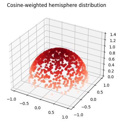
Cosine-weighted hemisphere sampling is implemented. The term \((\omega_i \cdot \mathrm{n})\) in the rendering equation equals \(\cos \theta\), where \(\theta\) is the zenith angle between the surface normal and the incoming ray direction. Directions which are close to perpendicular to the surface normal contribute very little light due to the cosine. It would be better to sample directions close to the surface normal.

The Monte Carlo estimator for non-uniform random variables \(X_i\) drawn out of probability density function (PDF) \(p(x)\) is

$$ F_n = \frac{1}{n} \sum_{i = 1}^{n} \frac{f(X_i)}{p(X_i)}. $$

Choosing \(p(\omega) = \frac{\cos \theta}{\pi}\) and, like before, taking just one sample, our estimator becomes:

$$ F_1 = \frac{\pi}{\cos \theta} f_{\textrm{lam}}L_i(\omega_i)(\omega_i \cdot \mathrm{n}). $$

We can substitute \((\omega_i \cdot \mathrm{n}) = \cos \theta\) and \(f_{\textrm{lam}} = \frac{k_{\textrm{albedo}}}{\pi}\) to simplify the estimator further:

$$ F_1 = k_{\textrm{albedo}}L_i(\omega_i), $$

where our light direction \(\omega_i\) is now drawn out of the cosine-weighted hemisphere. The code is simplified to just one function, which both samples the cosine-weighted direction and evaluates the albedo:

 1
 2
 3
 4
 5
 6
 7
 8
 9
10
11
12
13
14
15
16

struct Scatter {
    wi: vec3f,
    throughput: vec3f,
}

fn evalImplicitLambertian(hit: Intersection, rngState: ptr<function, u32>) -> Scatter {
    let v = rngNextInCosineWeightedHemisphere(rngState);
    let onb = pixarOnb(hit.n);
    let wi = onb * v;

    let textureDesc = textureDescriptors[textureDescriptorIndices[hit.triangleIdx]];
    let uv = hit.uv;
    let albedo = textureLookup(textureDesc, uv);

    return Scatter(wi, albedo);
}

Inverse transform sampling the cosine-weighted unit hemisphere.

The exact same recipe that was used for the unit hemisphere can be followed here to obtain rngNextInCosineWeightedHemisphere. While the recipe used is introduced in Physically Based Rendering, the book does not present this calculation.

Choice of PDF

Set probability density to be \(p(\omega) \propto \cos \theta\).

PDF normalization

Integrate \(p(\omega)\) over hemisphere H again.

$$ \int_H p(\omega) d\omega = \int_{0}^{2 \pi} \int_{0}^{\frac{\pi}{2}} c \cos \theta \sin \theta d\theta d\phi = \frac{c}{2} \int_{0}^{2 \pi} d\phi = 1 $$ $$ \Longrightarrow c = \frac{1}{\pi} $$

Coordinate transformation

Again, using the result \(p(\theta, , \phi) = \sin \theta p(\omega)\), obtain

$$ p(\theta , \phi) = \frac{1}{\pi} \cos \theta \sin \theta. $$

\(\theta\)’s marginal probability density

$$ p(\theta) = \int_{0}^{2 \pi} p(\theta , \phi) d \phi = \int_{0}^{2 \pi} \frac{1}{\pi} \cos \theta \sin \theta d \phi = 2 \sin \theta \cos \theta. $$

\(\phi\)’s conditional probability density

$$ p(\phi | \theta) = \frac{p(\theta , \phi)}{p(\theta)} = \frac{1}{2 \pi} $$

Calculate the CDF’s

$$ P(\theta) = \int_{0}^{\theta} 2 \cos \theta^{\prime} \sin \theta^{\prime} d \theta^{\prime} = 1 - \cos^2 \theta $$ $$ P(\phi | \theta) = \int_{0}^{\phi} \frac{1}{2 \pi} d\phi^{\prime} = \frac{\phi}{2 \pi} $$

Inverting the CDFs in terms of u

$$ \cos \theta = \sqrt{1 - u_1} = \sqrt{u_1} $$

$$ \phi = 2 \pi u_2 $$

where \(u_1 = 1 - u_1\) is substituted again. Converting \(\theta\), \(\phi\) back to Cartesian coordinates, note that \(z = \cos \theta = \sqrt{u_1}\).

$$ x = \sin \theta \cos \phi = \sqrt{1 - u_1} \cos(2 \pi u_2) $$ $$ y = \sin \theta \sin \phi = \sqrt{1 - u_1} \sin(2 \pi u_2) $$ $$ z = \sqrt{u_1} $$

In code:

 1
 2
 3
 4
 5
 6
 7
 8
 9
10
11
12
13

fn rngNextInCosineWeightedHemisphere(state: ptr<function, u32>) -> vec3f {
    let u1 = rngNextFloat(state);
    let u2 = rngNextFloat(state);

    let phi = 2f * PI * u2;
    let sinTheta = sqrt(1f - u1);

    let x = cos(phi) * sinTheta;
    let y = sin(phi) * sinTheta;
    let z = sqrt(u1);

    return vec3(x, y, z);
}

Looking at our duck, before:

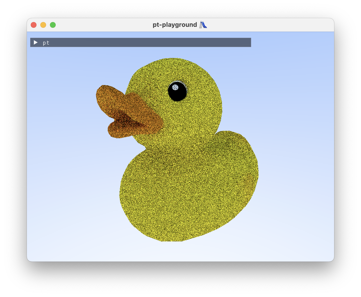
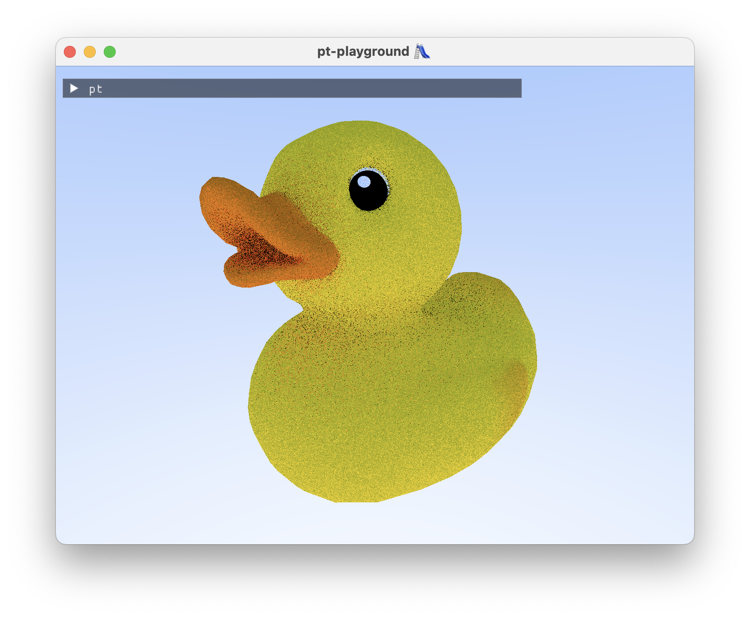
And after, with cosine-weighted hemisphere sampling:

The first physically-based pathtracer

2023-11-13

Commit: c83b83e

A simple physically-based pathtracer is implemented. ✨ The rendering equation is solved using the following Monte Carlo estimator:

$$ F_1 = 2 \pi f_r(\mathrm{x_i},\omega_i)L_i(\mathrm{x_i},\omega_i)(\omega_i\cdot\mathrm{n}), $$

where \(2 \pi\) is the surface area of the unit hemisphere, \(f_r\) is the bidirectional reflectance distribution function (BRDF), \(\omega_i\) is the incoming ray direction, and \(L_i\) is the incoming radiance along \(\omega_i\). The estimator is based on the Monte Carlo estimator for \(\int_{a}^{b} f(x) dx\), where the random variable is drawn from a uniform distribution:

$$ F_n = \frac{b-a}{n} \sum_{i=1}^{n} f(X_i), $$

where \(n=1\) is set for now and a surface area is used instead of the 1-dimensional range.

For simplicity, only the Lambertian BRDF is implemented at this stage, with \(f_{\textrm{lam}}=\frac{k_{\textrm{albedo}}}{\pi}\). Drawing inspiration from Crash Course in BRDF implementation, a pair of functions are implemented:

 1
 2
 3
 4
 5
 6
 7
 8
 9
10
11
12

fn sampleLambertian(hit: Intersection, rngState: ptr<function, u32>) -> vec3f {
    let v = rngNextInUnitHemisphere(rngState);
    let onb = pixarOnb(hit.n);
    return onb * v;
}

fn evalLambertian(hit: Intersection, wi: vec3f) -> vec3f {
    let textureDesc = textureDescriptors[textureDescriptorIndices[hit.triangleIdx]];
    let uv = hit.uv;
    let albedo = textureLookup(textureDesc, uv);
    return albedo * FRAC_1_PI * max(EPSILON, dot(hit.n, wi));
}

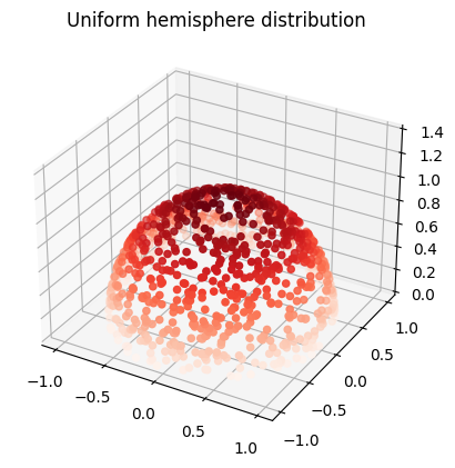
Inverse transform sampling the unit hemisphere.

To obtain rngNextInUnitHemisphere, we can follow a recipe introduced in Physically Based Rendering. Here’s a quick summary of the calculation, which is also partially in the book.

The recipe

In order to do Monte Carlo integration, you will need to do inverse transform sampling with your selected probability density function (PDF). Here’s the general steps that you need to take to arrive at a function that you can use to draw sampels from.

1. Choose the probability density function.
2. If the density function is multidimensional, you can compute the marginal density (integrate out one variable), and the conditional density for the other variable.
3. Calculate the cumulative distribution function (CDF).
4. Invert the CDFs in terms of the canonical uniform random variable, \(u\).

Choice of PDF

Uniform probability density over all directions \(\omega\), \(p(\omega) = c\).

PDF normalization

The integral over the hemisphere H yields the surface area of a hemisphere:

$$ \int_{H} c d \omega = 2 \pi c = 1 $$

$$ c = \frac{1}{2 \pi} $$

Coordinate transformation

Use the result that \(p(\theta, , \phi) = \sin \theta p(\omega)\) to obtain

$$ p(\theta , \phi) = \frac{\sin \theta}{2 \pi} $$

\(\theta\)’s marginal probability density

$$ p(\theta) = \int_{0}^{2 \pi} p(\theta , \phi) d \phi = \int_{0}^{2 \pi} \frac{\sin \theta}{2 \pi} d \phi = \sin \theta $$

\(\phi\)’s conditional probability density

In general, \(\phi\)’s probability density would be conditional on \(\theta\) after computing \(\theta\)’s marginal density.

$$ p(\phi | \theta) = \frac{p(\theta , \phi)}{p(\theta)} = \frac{1}{2 \pi} $$

Calculate the CDF’s

$$ P(\theta) = \int_{0}^{\theta} \sin \theta^{\prime} d\theta^{\prime} = 1 - \cos \theta $$

$$ P(\phi | \theta) = \int_{0}^{\phi} \frac{1}{2 \pi} d\phi^{\prime} = \frac{\phi}{2 \pi} $$

Inverting the CDFs in terms of u

$$ \theta = \cos^{-1}(1 - u_1) $$

$$ \phi = 2 \pi u_2 $$

\(u_1 = 1 - u_1\) can be substituted as it is just another canonical uniform distribution, to obtain

$$ \theta = \cos^{-1}(u_1) $$

$$ \phi = 2 \pi u_2 $$

Convert \(\theta\) and \(\phi\) back to Cartesian coordinates

$$ x = \sin \theta \cos \phi = \sqrt{1 - u_1^2} \cos(2 \pi u_2) $$ $$ y = \sin \theta \sin \phi = \sqrt{1 - u_1^2} \sin(2 \pi u_2) $$ $$ z = u_1 $$

where we used the identity \(\sin \theta = \sqrt{1 - \cos^2 \theta}\). In code:

 1
 2
 3
 4
 5
 6
 7
 8
 9
10
11
12
13

fn rngNextInUnitHemisphere(state: ptr<function, u32>) -> vec3f {
    let u1 = rngNextFloat(state);
    let u2 = rngNextFloat(state);

    let phi = 2f * PI * u2;
    let sinTheta = sqrt(1f - u1 * u1);

    let x = cos(phi) * sinTheta;
    let y = sin(phi) * sinTheta;
    let z = u1;

    return vec3(x, y, z);
}

It generates unit vectors, distributed uniformly in a hemisphere about the z axis.

The functions are used in the path-tracing loop as follows:

 1
 2
 3
 4
 5
 6
 7
 8
 9
10
11
12
13
14
15
16
17
18
19
20
21
22
23
24
25

const UNIFORM_HEMISPHERE_MULTIPLIER = 2f * PI;

fn rayColor(primaryRay: Ray, rngState: ptr<function, u32>) -> vec3f {
    var ray = primaryRay;

    var color = vec3(0f);
    var throughput = vec3(1f);
    for (var bounces = 0u; bounces < NUM_BOUNCES; bounces += 1u) {
        var intersection: Intersection;
        if rayIntersectBvh(ray, T_MAX, &intersection) {
            let p = intersection.p;
            let scatterDirection = sampleLambertian(intersection, rngState);
            let scatterThroughput =
                UNIFORM_HEMISPHERE_MULTIPLIER * evalLambertian(intersection, scatterDirection);
            ray = Ray(p, scatterDirection);
            throughput *= scatterThroughput;
        } else {
            // compute sky color
            ...
            break;
        }
    }

    return color;
}

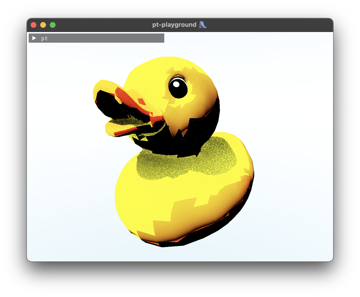
We can now pathtrace our duck. If the noise on the duck exhibits a grid-like pattern, you should open the full-size image as the website scales the images down.

Now that real work is being done in the shader, the performance of Sponza on my M2 Macbook Air is starting to become punishing. Framerates are in the 1-10 FPS range with the depicted image sizes.

Simple texture support 🖼️

2023-11-10

Commit: 8062be7

Initial textures support is added. The “base color texture” from the glTF “pbr metallic roughness” material is loaded and passed over to the GPU. The same storage buffer approach from my Weekend raytracing with wgpu, part 2 post is used for texture lookup on the GPU.

1
2
3
4
5
6
7
8

// Each triangle is associated with an index to a texture descriptor, a
// placeholder for a texture on the GPU.
@group(2) @binding(4) var<storage, read_write> textureDescriptorIndices: array<u32>;
// A texture descriptor contains an offset into the texture buffer, as
// well as the texture dimensions.
@group(2) @binding(5) var<storage, read_write> textureDescriptors: array<TextureDescriptor>;
// The texture buffer contains textures from all meshes, appended end to end.
@group(2) @binding(6) var<storage, read_write> textures: array<u32>;

On ray-triangle intersection, the model vertex UV coordinates are interpolated and the color is computed from the corresponding texel.

 1
 2
 3
 4
 5
 6
 7
 8
 9
10
11
12
13
14
15
16
17
18
19
20
21

if rayIntersectBvh(ray, T_MAX, &intersection, &triangleIdx) {
    let textureDesc = textureDescriptors[textureDescriptorIndices[triangleIdx]];
    
    let b = intersection.b;
    let uvs = texCoords[triangleIdx];
    let uv = b[0] * uvs[0] + b[1] * uvs[1] + b[2] * uvs[2];

    color = textureLookup(textureDesc, uv);
}

fn textureLookup(desc: TextureDescriptor, uv: vec2f) -> vec3f {
    let u = clamp(uv.x, 0f, 1f);
    let v = clamp(uv.y, 0f, 1f);

    let j = u32(u * f32(desc.width));
    let i = u32(v * f32(desc.height));
    let idx = i * desc.width + j;

    let rgba = textures[desc.offset + idx];
    return vec3f(f32(rgba & 0xffu), f32((rgba >> 8u) & 0xffu), f32((rgba >> 16u) & 0xffu)) / 255f;
}

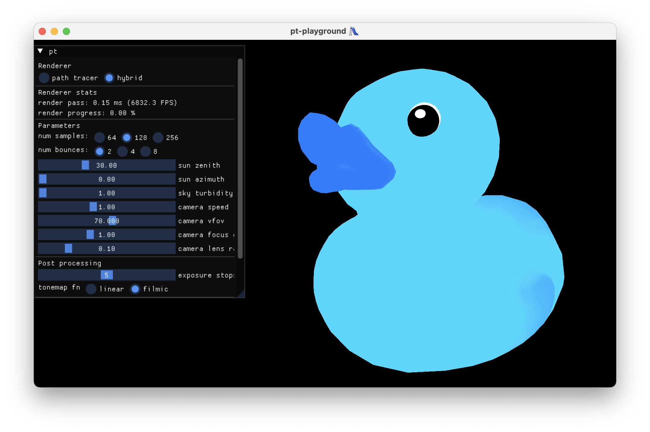
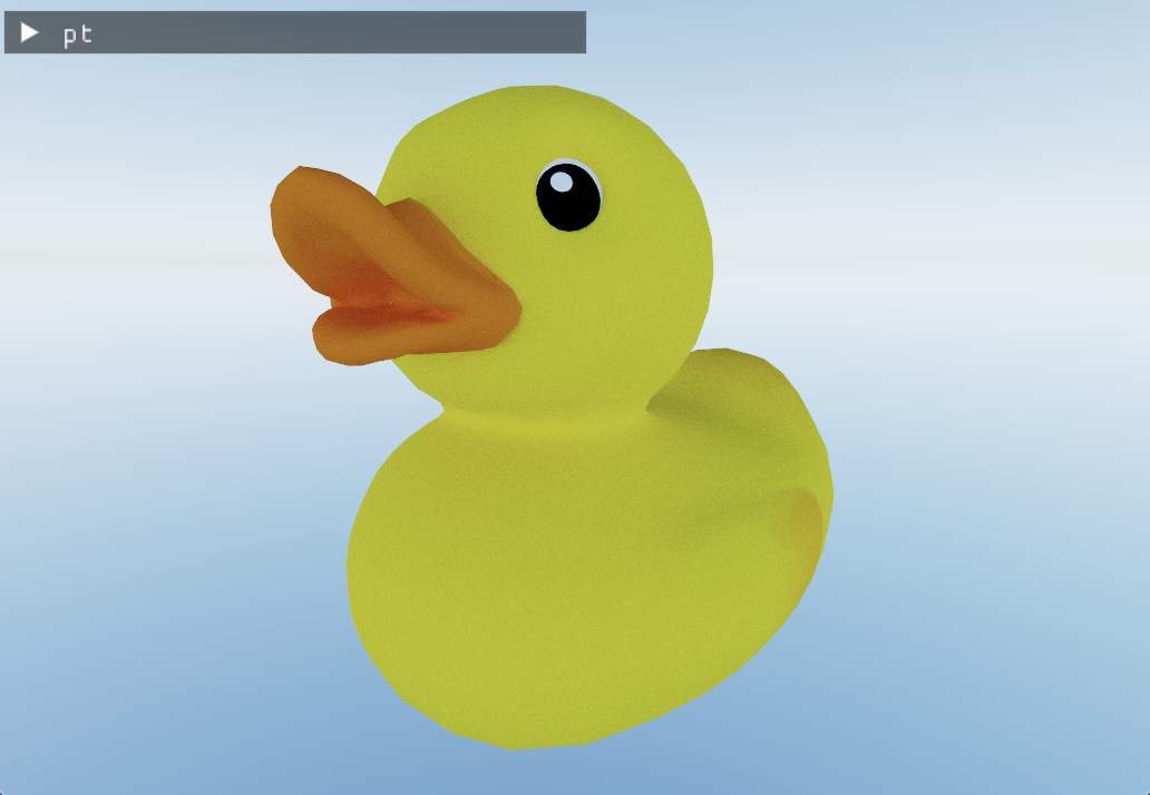
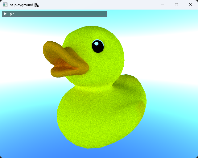
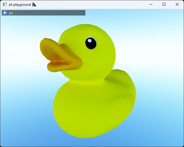
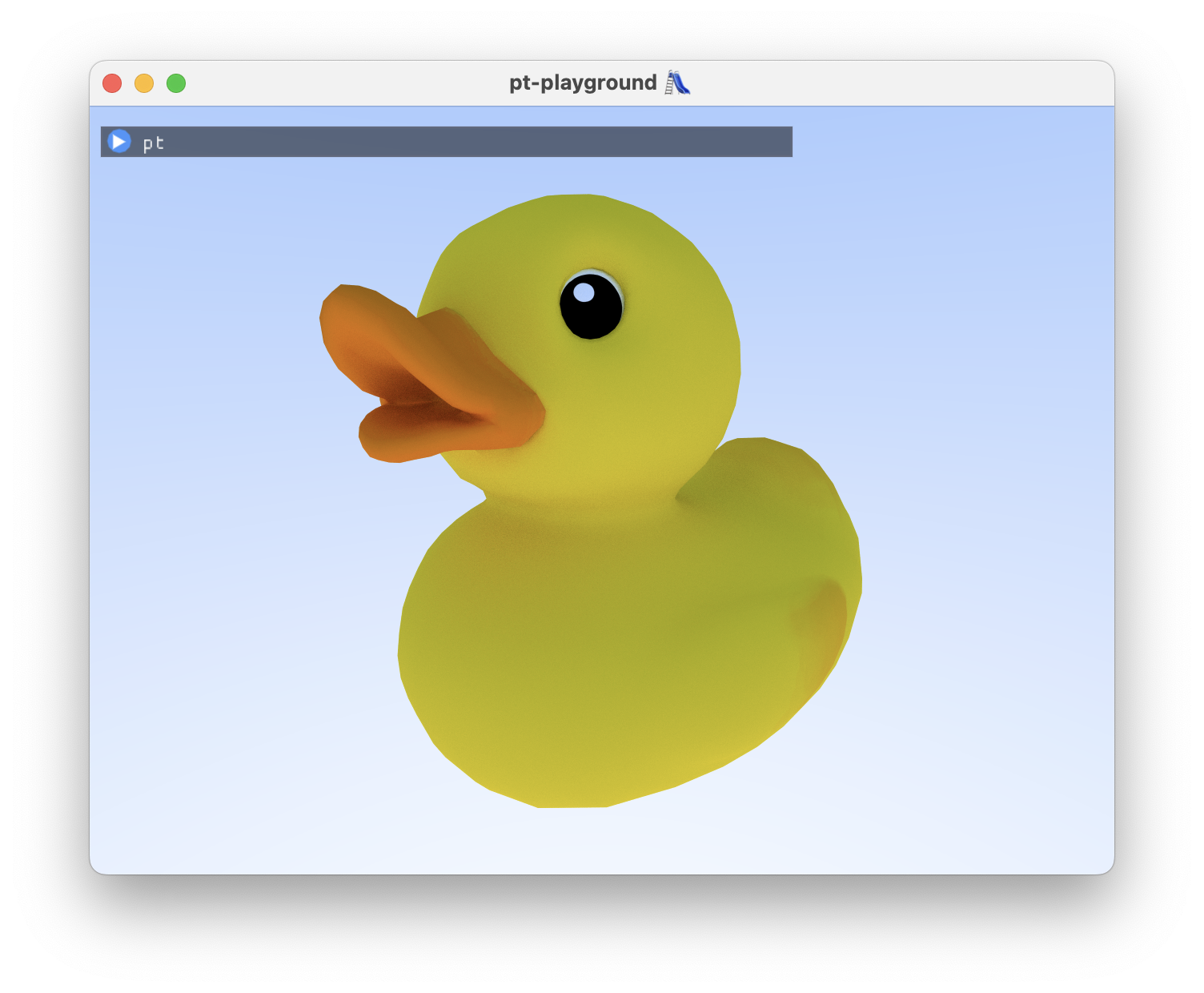
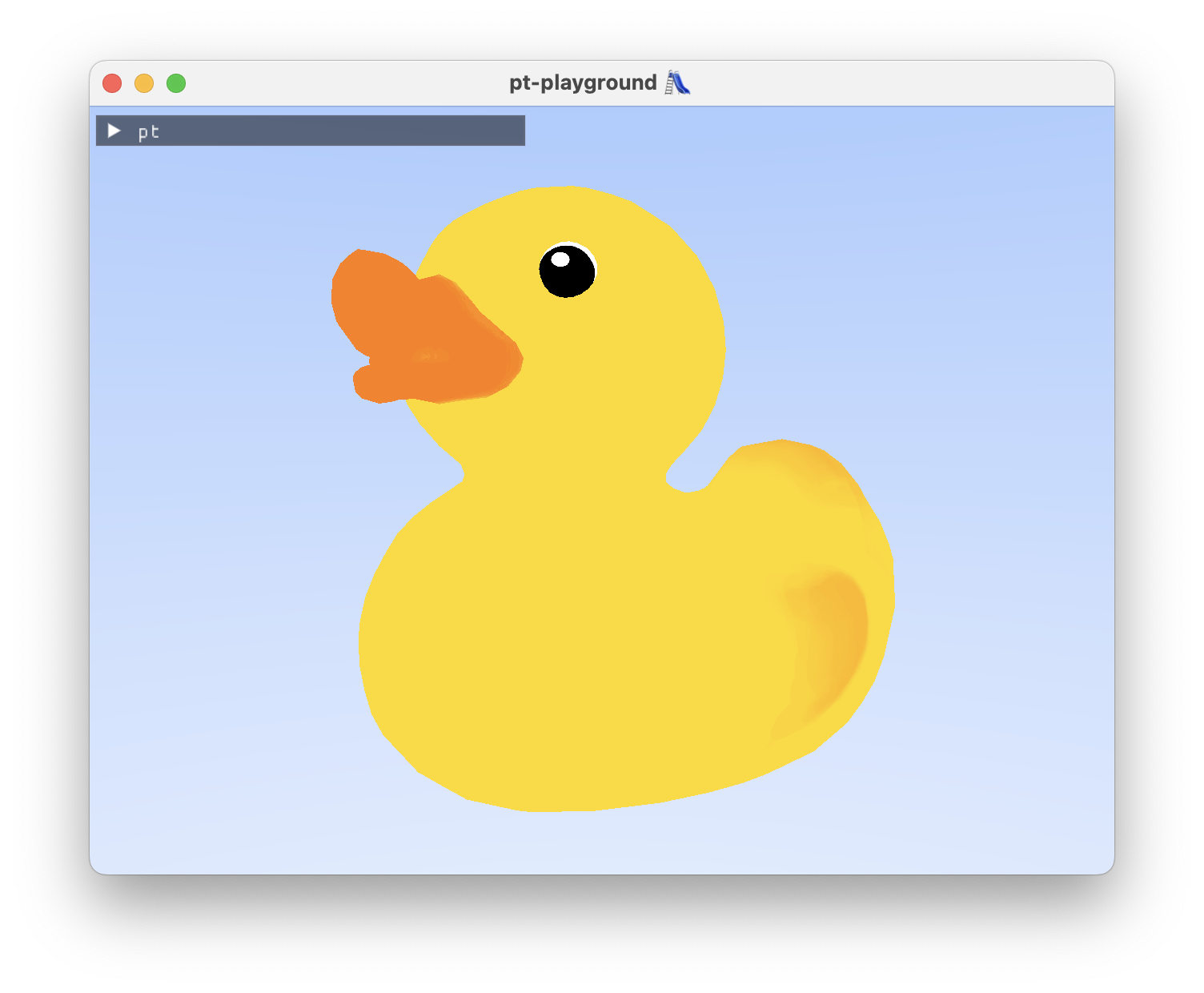
The duck model from earlier looks more like a rubber duck now.

Sponza looks a bit rough at this stage. Two things need work.

• The plants in the foreground need transparency support. On intersection, the transparency of the pixel also needs to be accounted for the ray to intersect the triangle.
• There is an issue with the textures on the ground and in some places on the walls being stretched out.

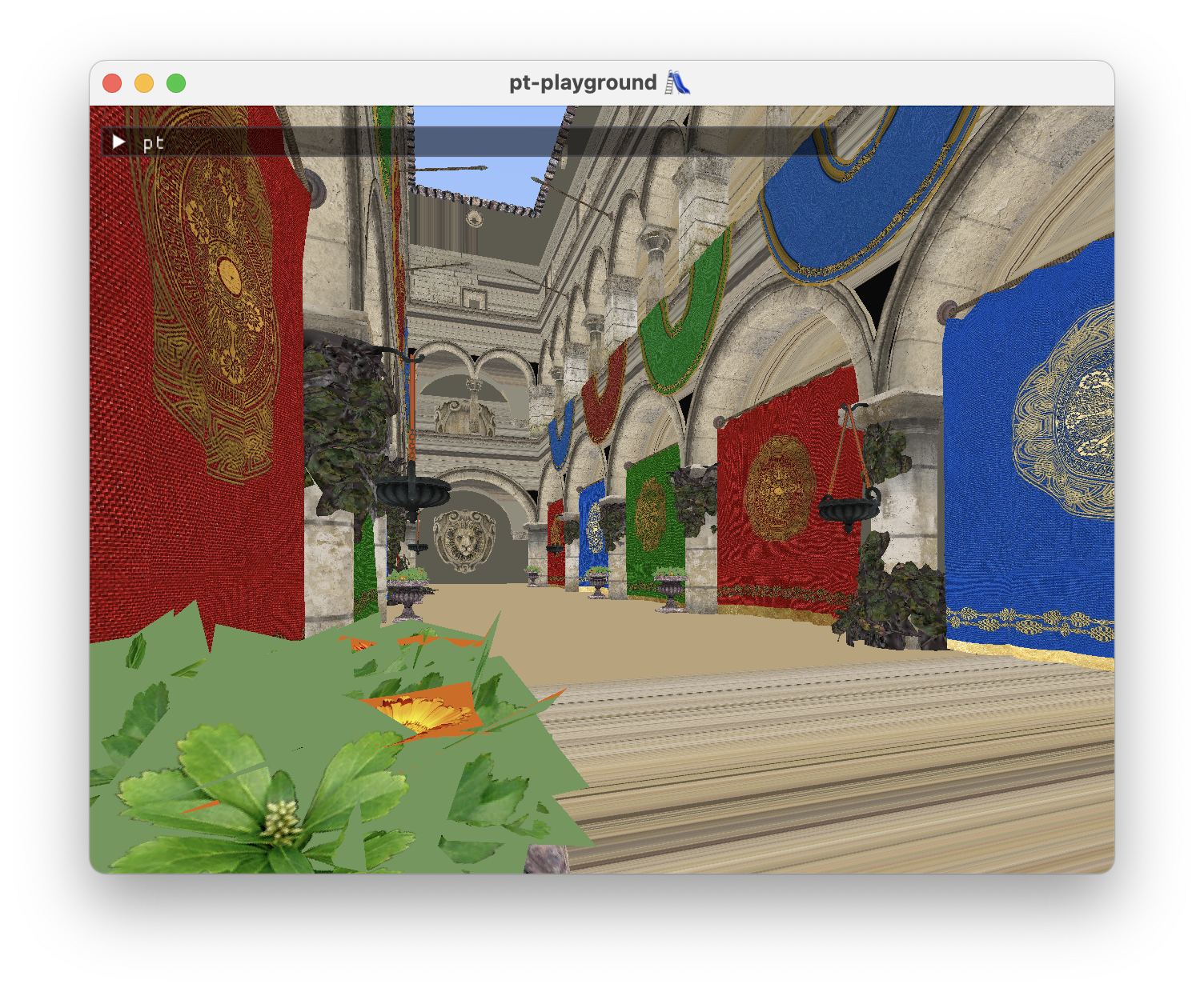
The stretched textures are likely due to a problem with UV coordinate interpolation. Single colors and suspicious red-black color gradients can be seen when coloring the model according to the triangles’ interpolated UV coordinates.

Interpolated normals, texture coordinates, and GPU timers

2023-11-09

Commit: 82208c1

GPU timers

Timing the render pass on the device timeline allows us to keep track of how long rendering the scene actually takes on the GPU, no matter what I do on the CPU side. The timings are displayed in the UI as a moving average.

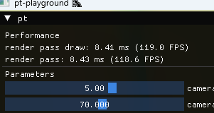
My 3080 RTX currently runs the Sponza atrium scene (see below) at roughly 120 FPS at fullscreen resolutions.

Enabling allow-unsafe-apis

WebGPU timestamp queries are disabled by default due to timings being potentially usable for client fingerprinting. Using the timestamp queries requires toggling “allow-unsafe-apis” (normally toggled via Chrome’s settings) using the WebGPU native’s struct extension mechanism:

 1
 2
 3
 4
 5
 6
 7
 8
 9
10
11
12
13
14
15
16

const char*               allowUnsafeApisToggle = "allow_unsafe_apis";
WGPUDawnTogglesDescriptor instanceToggles = {
    .chain =
        WGPUChainedStruct{
            .next = nullptr,
            .sType = WGPUSType_DawnTogglesDescriptor,
        },
    .enabledTogglesCount = 1,
    .enabledToggles = &allowUnsafeApisToggle,
    .disabledTogglesCount = 0,
    .disabledToggles = nullptr,
};
const WGPUInstanceDescriptor instanceDesc{
    .nextInChain = &instanceToggles.chain,
};
const WGPUInstance instance = wgpuCreateInstance(&instanceDesc);

Loading normals and texture coordinates, triangle interpolation

The model surface normals and texture coordinates are loaded from the model. The model now exposes arrays of vertex attributes:

 1
 2
 3
 4
 5
 6
 7
 8
 9
10
11
12
13
14
15
16
17

class GltfModel
{
public:
    GltfModel(std::filesystem::path gltfPath);

    std::span<const Positions>   positions() const { return mPositions; }
    std::span<const Normals>     normals() const { return mNormals; }
    std::span<const TexCoords>   texCoords() const { return mTexCoords; }
    std::span<const std::size_t> baseColorTextureIndices() const
    {
        return mBaseColorTextureIndices;
    }
    std::span<const Texture> baseColorTextures() const { return mBaseColorTextures; }

private:
    ...
};

Normals and texture coordinates are interpolated at the intersection point using the intersection’s barycentric coordinates:

1
2
3
4
5
6
7

if rayIntersectBvh(ray, T_MAX, &intersection, &triangleIdx) {
    let b = intersection.b;

    let tnorms = normals[triangleIdx];
    let n = b[0] * tnorms[0] + b[1] * tnorms[1] + b[2] * tnorms[2];
    color = 0.5f * (vec3f(1f, 1f, 1f) + n);
}

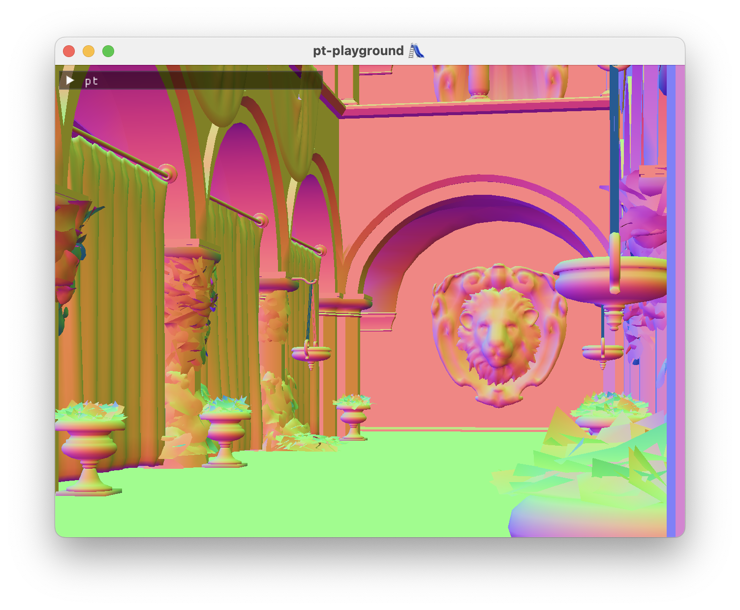
Here’s the famous Sponza atrium scene demonstrating the smoothly interpolated normals:

Loading textures

2023-11-08

Commit: 1706265

The glTF model loader now loads textures, and the base color textures are exposed in the model:

 1
 2
 3
 4
 5
 6
 7
 8
 9
10
11
12
13
14
15

class GltfModel
{
public:
    GltfModel(std::filesystem::path gltfPath);

    std::span<const Triangle>    triangles() const { return mTriangles; }
    std::span<const std::size_t> baseColorTextureIndices() const
    {
        return mBaseColorTextureIndices;
    }
    std::span<const Texture> baseColorTextures() const { return mBaseColorTextures; }

private:
    ...
};

Each triangle has a base color texture index, and it can be used to index into the array of base color textures. Textures are just arrays of floating point values.

A new textractor executable (short for texture extractor 😄) is added. It loads a GLTF model, and then dumps each loaded texture into a .ppm file. This way, it can be visually inspected that the textures have been loaded correctly. For instance, here is the duck model’s base_color_texture_0:

Camera and UI interaction

2023-11-07

Commit: 1593e8a

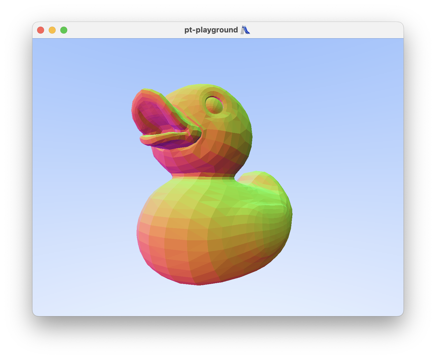
In order to work with arbitrary 3d models, camera positions and parameters should not be hard-coded. To kickstart scene interaction, two things are implemented:

• A “fly camera”, which allows you to move around and pan the scene around using the mouse.
• A UI integration, and a panel which allows you to edit the camera’s speed, and vfov.

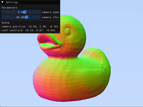
The UI panel also prints out scene debug information:

1
2
3

Scene
camera position: (8.00, 2.80, -8.30)
root centroid: (0.13, 0.87, -0.04)

A bug with the model loader’s model transform meant that the duck was hundreds of units away from the camera vertically. Without the debug UI, it was hard to tell whether I just couldn’t find the model in space, or whether the camera controller had a problem.

Raytracing triangles on the GPU 🎉

2023-11-06

Commit: e950ea8

Today’s achievement:

The BVH and all intersection testing functions are ported to the shader. The rays from the previous devlog entry are now directly used against the BVH.

Porting the BVH to the GPU involved adjusting the memory layout of a number of structs. Triangles, Aabbs, and the BvhNodes all have vectors in them which need to be 16-byte aligned in memory. This was achieved by padding the structs out. E.g. BvhNode,

 1
 2
 3
 4
 5
 6
 7
 8
 9
10
11
12
13
14
15
16
17
18
19

-struct BvhNode
-{
-    Aabb aabb;                   // offset: 0, size: 24
-    union
-    {
-        std::uint32_t trianglesOffset;
-        std::uint32_t secondChildOffset;
-    };                           // offset: 24, size: 4
-    std::uint16_t triangleCount; // offset: 28, size: 2
-    std::uint16_t splitAxis;     // offset: 30, size: 2
-};
+struct BvhNode
+{
+    Aabb32        aabb;              // offset: 0, size: 32
+    std::uint32_t trianglesOffset;   // offset: 32, size: 4
+    std::uint32_t secondChildOffset; // offset: 36, size: 4,
+    std::uint32_t triangleCount;     // offset: 40, size: 4
+    std::uint32_t splitAxis;         // offset: 44, size: 4
+};

I also tried using AI (GitHub Copilot) to translate some of the hundreds of lines of intersection testing code to WGSL. It worked well in the sense that only certain patterns of expression had to be fixed. I likely avoided errors that I would have introduced manually porting the code over.

🤓 TIL about the @must_use tag in WGSL. It’s used as an annotation for functions which return values and don’t have side effects. Not using the function in assignment or an expression becomes a compile error.

1
2
3
4

@must_use
fn rayPointAtParameter(ray: Ray, t: f32) -> vec3f {
    return ray.origin + t * ray.direction;
}

Raytracing spheres on the GPU

2023-11-04

Commit: 16f6255

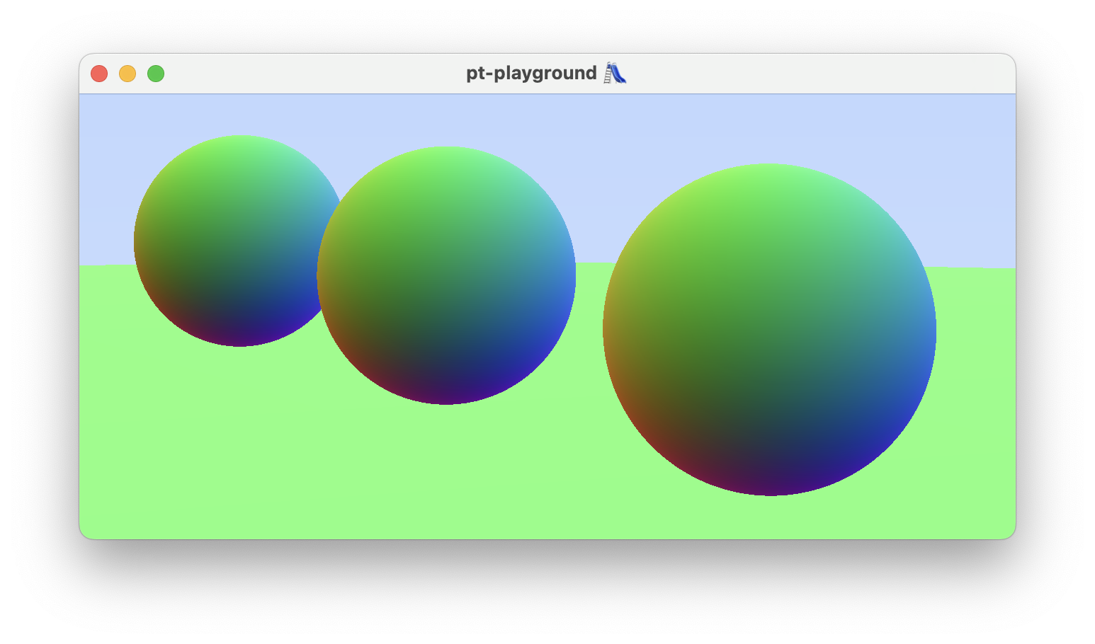
Before attempting to raytrace triangles on the GPU, first I need to demonstrate that the camera actually works in the shader.

To do so, a simple raytracing scenario is first implemented. An array of spheres, stored directly in the shader is added. Ray-sphere intersection code is copied over from my weekend-raytracer-wgpu project. The spheres are colored according to their surface normal vector. The spheres are visible and now I know that the camera works!

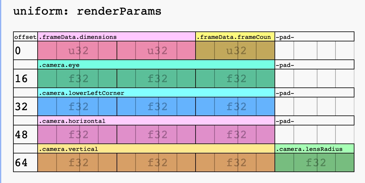
The camera and the frame data struct are bundled together into on uniform buffer.

 1
 2
 3
 4
 5
 6
 7
 8
 9
10
11
12
13
14
15
16
17

struct RenderParams {
  frameData: FrameData,
  camera: Camera,
}

struct FrameData {
  dimensions: vec2u,
  frameCount: u32,
}

struct Camera {
  eye: vec3f,
  lowerLeftCorner: vec3f,
  horizontal: vec3f,
  vertical: vec3f,
  lensRadius: f32,
}

I used WGSL Offset Computer, a great online resource for enumerating and drawing the memory layout of your WGSL structs, as a sanity check that my memory layout for renderParams was correct.

Hello, bounding volume hierarchies

2023-11-02

Commit: 624e5ea

This entry marks the first step towards being able to shoot rays at complex triangle geometry. A bounding volume hierarchy (BVH) is introduced (common/bvh.hpp) and tested.

The test (tests/bvh.cpp) intersects rays with the BVH, and uses a brute-force test against the full array of triangles as the ground truth. The intersection test result (did intersect or did not) and the intersection point, in the case of intersection, must agree for all camera rays in order for the test to pass.

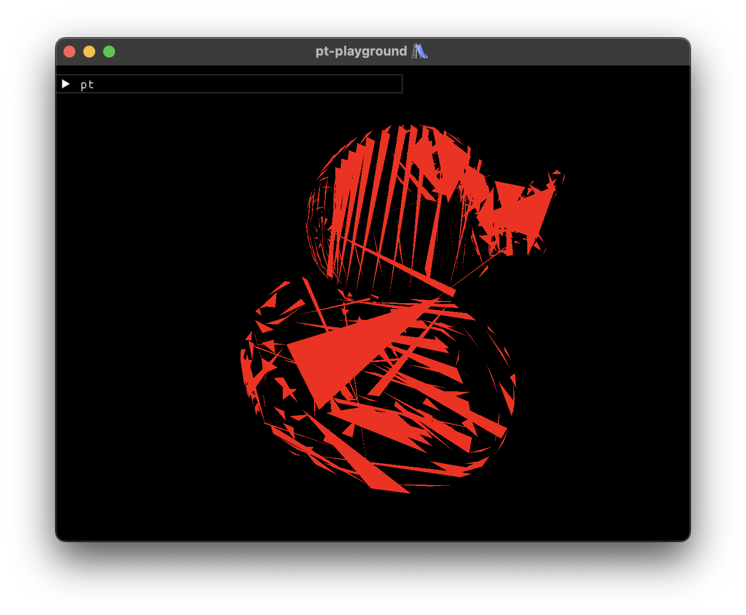
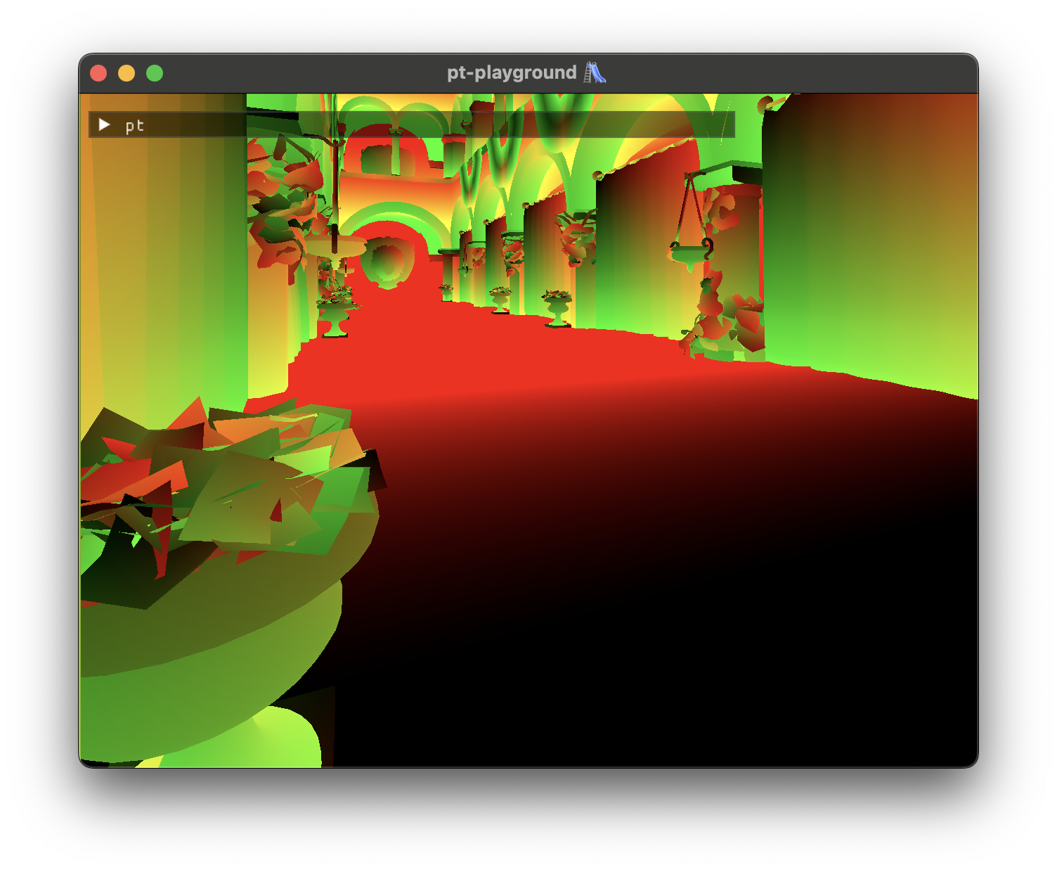
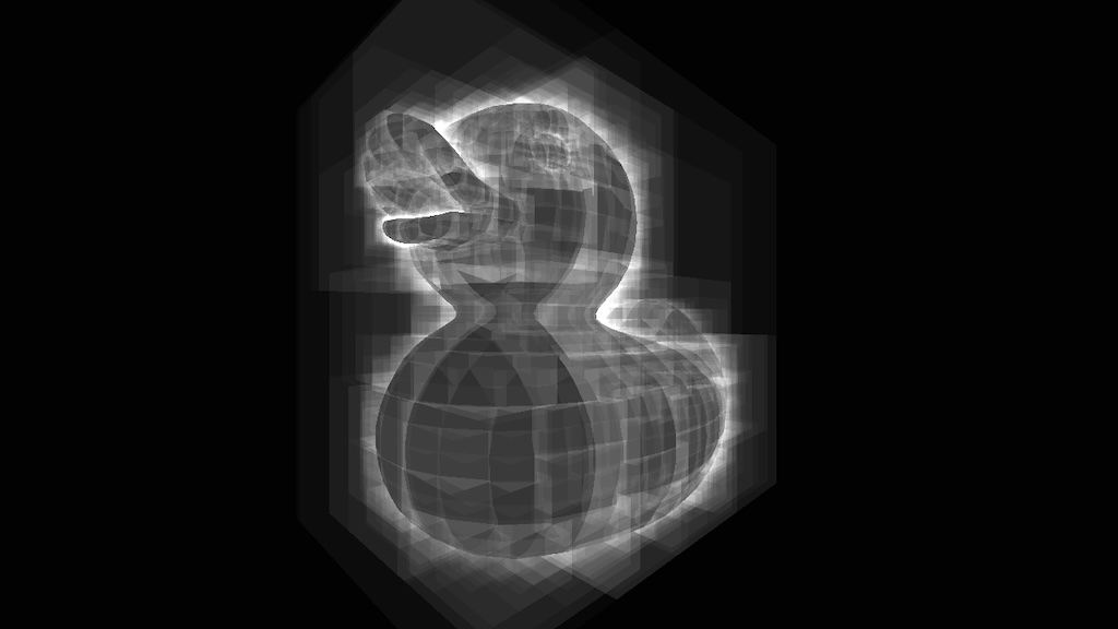
As an additional end-to-end sanity check, a new executable target (bvh-visualizer) is introduced. Primary camera rays are generated and the number of BVH nodes visited per ray is visualized as an image.

GpuBuffer

2023-11-01

Commit: 0a826c4

Not a lot of visible progress, but GpuBuffer was introduced (in gpu_buffer.hpp) to significantly reduce the amount of boilerplate due to buffers & bind group descriptors:

Showing 5 changed files with 254 additions and 275 deletions.

On another note, used immediately invoked lambda functions in a constructor initializer for the first time today:

 1
 2
 3
 4
 5
 6
 7
 8
 9
10
11
12
13

Renderer::Renderer(const RendererDescriptor& rendererDesc, const GpuContext& gpuContext)
    : frameDataBuffer(...),
      pixelBuffer(
          gpuContext.device,
          "pixel buffer",
          WGPUBufferUsage_CopyDst | WGPUBufferUsage_Storage,
          [&rendererDesc]() -> std::size_t {
              const Extent2i    largestResolution = rendererDesc.maxFramebufferSize;
              const std::size_t numPixels =
                  static_cast<std::size_t>(largestResolution.x * largestResolution.y);
              return sizeof(glm::vec3) * numPixels;
          }()),
      ...

It’s busy looking, but it enables you to do actual work in the constructor initializer. Doing all the work in the constructor initializers like this could make move constructors unnecessary.

GPU-generated noise

2023-10-31

Commit: 645c09c

The major highlights of the day include generating noise on the GPU and displaying it, as well as cleaning up the main function using a new Window abstraction.

Window

A simple Window abstraction is introduced to automate GLFW library and window init and cleanup. main does not yet have an exception handler, but this abstraction is a step closer to ensuring all resources are cleaned up even when exceptions occur.

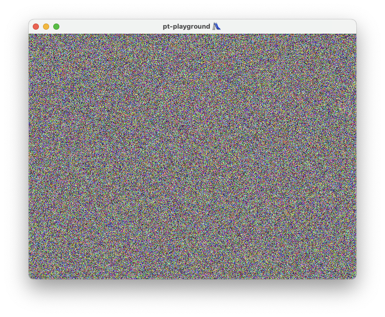
GPU noise

Noise is generated on the GPU using the following functions.

 1
 2
 3
 4
 5
 6
 7
 8
 9
10
11
12
13

fn rngNextFloat(state: ptr<function, u32>) -> f32 {
    let x = rngNextInt(state);
    return f32(x) / f32(0xffffffffu);
}

fn rngNextInt(state: ptr<function, u32>) {
    // PCG random number generator
    // Based on https://www.shadertoy.com/view/XlGcRh
    let newState = *state * 747796405u + 2891336453u;
    *state = newState;
    let word = ((newState >> ((newState >> 28u) + 4u)) ^ newState) * 277803737u;
    return (word >> 22u) ^ word;
}

NOTE: A reader pointed out that the implementation contained in the linked commit is incorrect. The functions listed above are the correct implementation of a PCG random number generator.

Each frame,

1. rngNextFloat is used in a compute shader to generate RGB values
2. RGB values are stored in a pixel buffer
3. The pixel buffer is mapped to the full screen quad from the previous day.

This approach is a bit more complex than necessary, and could just be done in the fragment shader.

Fullscreen quad

2023-10-30

Commit: 51387d7

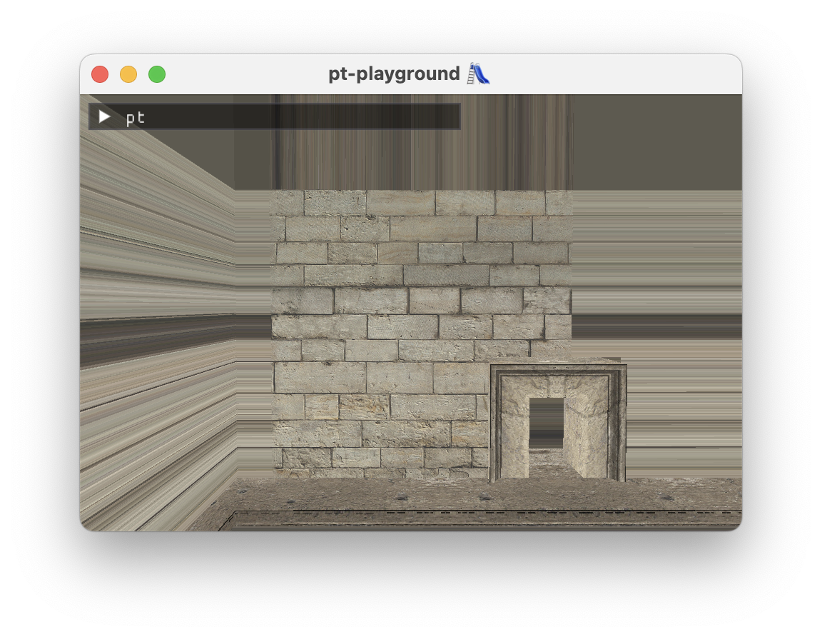
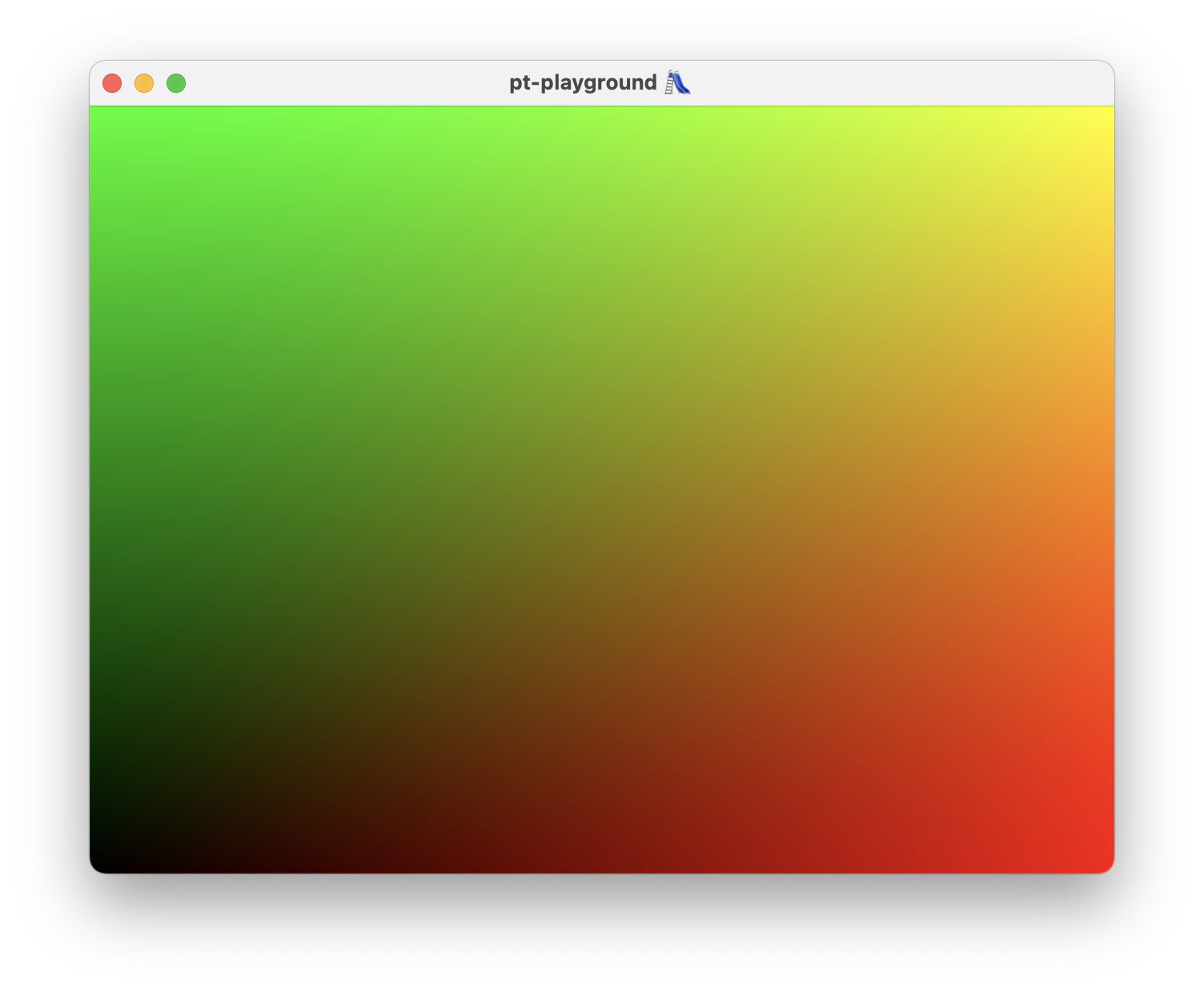
After 1000 lines of WebGPU plumbing code, the first pair of triangles is displayed on the screen in the shape of a fullscreen quad, and the UV coordinates are displayed as a color.

The pt executable contains

• A GpuContext for initializing the WebGPU instance, surface, adapter, device, queue, and the swap chain.
• A distinct Renderer which initializes a render pipeline, a uniform and vertex buffer, using the GpuContext.

The renderer draws to the screen using a fullscreen quad. For now, the texture coordinates are displayed as colors.

Hello, GLFW!

2023-10-29

Commit: 4df39fa

All projects have to start somewhere.

• Defined a pt executable target in CMake. The goal is for this executable to open up a scene and display it by doing pathtracing on the GPU.
• The GLFW library dependency added using CMake’s FetchContent.
• An empty window is opened with a window title. No GPU rendering support yet, only calls to glfwSwapBuffers.

A windows opens with a black frame.