Weekend raytracing with wgpu, part 2

The first part of “Weekend raytracing with wgpu” left us with a basic implementation of Peter Shirley’s first book in the series of “Ray Tracing In One Weekend " books. “Ray Tracing: The Next Week” introduces additional features, such as texture support.

This post takes a look at adding a physically based sky model, in addition to adding textured material support. These features, combined, result in much nicer images than the basic renderer, without appreciably slowing down the renderer. Adding textures was not as simple as porting the code over from the book as the book’s OOP-heavy approach does not map easily to a GPU.

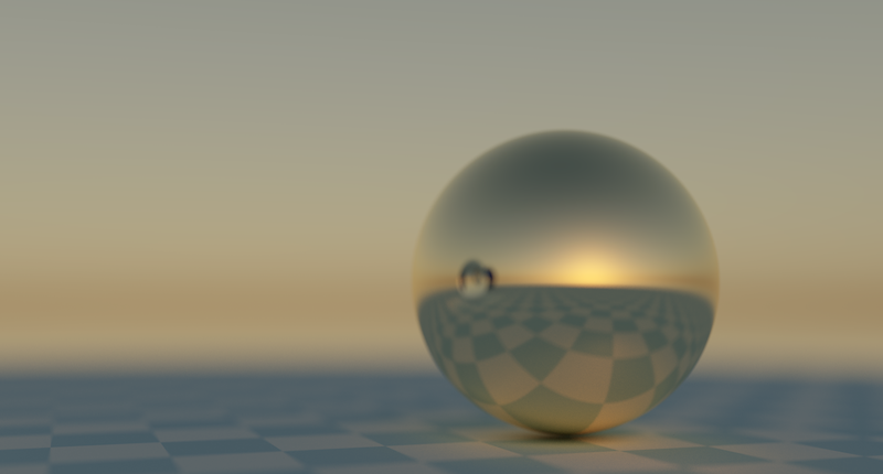
Unlike the previous post, where the sky color was an almost flat shade of blue, we now have an actual light source in the scene, the sun. This leads to emergent visual features, which didn’t have to be implemented separately. Notice the light reflected off the gold orb onto the checkerboard pattern in the image below. As you rotate the sun around the orb, you can watch the reflection move in real-time. Nothing was changed in the way the rays bounce off the spheres, the spheres are simple reflecting a much higher quality sky.

Adding a physically-based sky model

There are many sky models to choose from, all with distinct goals and use-cases in mind. The sky model I chose was the Hosek-Wilkie model. It looks good enough for the weekend raytracer project and is easy to integrate in a raytracer, regardless of whether you are rendering on the GPU or the CPU.

The model provides physically-based radiance values for any direction in the sky, assuming the viewer is on the ground of the Earth. The model was obtained by doing brute-force simulations of the atmospheric scattering process on Earth, and then fitting the results into a simple model that is much faster to evaluate at runtime.

Integrating the Hosek-Wilkie model

Evaluating the sky model (i.e. calculating the radiance for a viewing direction) involves doing some calculations using a lookup table. If you change a sky parameter, such as the sun direction or the atmospheric turbidity, the table values will need to be recomputed.

The authors behind the original paper provide a reference C implementation, which can be used a basis of an integration. However, the fastest way to get the model integrated in a Rust-based renderer is to use the hw-skymodel crate. This crate only supports RGB radiances, simplifying runtime evaluation and calculation of the table values.

To summarize, using the hw-skymodel crate involves two steps: generating the lookup table values, and using the radiance function to calculate the radiance for any given viewing direction at runtime.

The table values and sun direction are contained the raytracer’s SkyState struct.

1
2
3
4
5

struct SkyState {
    params: array<f32, 27>,
    radiances: array<f32, 3>,
    sunDirection: vec3<f32>,
};

The raytracer’s radiance function is copy-pasted from the crate. Rust and WGSL are similar enough that it takes just a few minutes to fix syntactical differences. With this setup, all you have to do is upload the SkyState data on initialization and any time sky parameters change. The hw-skymodel crate’s SkyState::new function is fast enough that you can call it at runtime to regenerate the lookup table.

In order to call the radiance function, you need to provide information about the view direction. Two angles are required: theta, the polar angle of the view vector, and gamma, the angle between the view vector and the sun direction. Here is one way those can be computed:

 1
 2
 3
 4
 5
 6
 7
 8
 9
10
11

let v = normalize(ray.direction);
let s = skyState.sunDirection;

let theta = acos(v.y);
let gamma = acos(clamp(dot(v, s), -1f, 1f));

color = vec3(
    radiance(theta, gamma, channelR),
    radiance(theta, gamma, channelG),
    radiance(theta, gamma, channelB)
);

channelR, channelG, channelB are constant values representing the channel index.

To see everything in context, you can read the rayColor function where the sky model is evaluated in the ray miss branch.

Adding tonemapping

The sky model outputs physical radiance values, which are not contained in the 0, 1 range. Without a tone mapping function, the image will be completely white.

A tone mapping function applies a curve to the raw radiance value, to map it to the 0, 1 range. The glsl-tone-map page contains a gallery of different functions you can use. I found that the uncharted2 function looked the best in the weekend-raytracer scene, so I chose that. Note that the example code’s exposureBias = 2.0 yielded an image which was too bright. A value of 0.246 worked much better.

 1
 2
 3
 4
 5
 6
 7
 8
 9
10
11
12
13
14
15
16
17
18
19

fn uncharted2(x: vec3<f32>) -> vec3<f32> {
    let exposureBias = 0.246;   // determined experimentally for the scene
    let curr = uncharted2Tonemap(exposureBias * x);

    let w = 11.2;
    let whiteScale = 1f / uncharted2Tonemap(vec3(w));
    return whiteScale * curr;
}

fn uncharted2Tonemap(x: vec3<f32>) -> vec3<f32> {
    let a = 0.15;
    let b = 0.50;
    let c = 0.10;
    let d = 0.20;
    let e = 0.02;
    let f = 0.30;
    let w = 11.2;
    return ((x*(a*x+c*b)+d*e)/(x*(a*x+b)+d*f))-e/f;
}

To tone map your image, you simply pass each RGB value through the function.

1
2
3
4
5

let invN = 1f / f32(samplingParams.accumulatedSamplesPerPixel);
return vec4(
        uncharted2(invN * pixel),
        1f
    );

Adding texture support

Unlike rasterization, where you render one object at a time, in raytracing the ray may hit any object in the scene. We already retain all our spheres in memory, and we will have to do the same for the textures, which once again means that we need to ignore WebGPU’s built-in texture support and implement our own system.

UV coordinates

First, in order to map a texture to a sphere’s surface, we need a way to generate UV coordinates for ever ray-sphere intersection. The updated sphereIntersection function generates uv coordinates for any intersection on the surface of a sphere. This implementation is straight out of the Ray Tracing: The Next Week book.

 1
 2
 3
 4
 5
 6
 7
 8
 9
10

fn sphereIntersection(ray: Ray, sphere: Sphere, t: f32) -> Intersection {
    let p = rayPointAtParameter(ray, t);
    let n = (1f / sphere.radius) * (p - sphere.centerAndPad.xyz);
    let theta = acos(-n.y);
    let phi = atan2(-n.z, n.x) + pi;
    let u = 0.5 * frac1Pi * phi;
    let v = frac1Pi * theta;

    return Intersection(p, n, u, v, t);
}

Now that we have rectangular UV coordinates for our surface, we can do a texture lookup using the UV coordinates.

Texture storage and lookup

All textures are stored in a single array, back to back. Texels are an array<f32,3>, instead of a vec3<f32> to avoid the 16-byte memory alignment requirement that a vec3 would require. This way, the textures consume less memory.

@group(3) @binding(2) var<storage, read> textures: array<array<f32, 3>>;

The texture object contains the dimensions of the texture, as well as the texture’s offset into the global texture storage array.

1
2
3
4
5

struct TextureDescriptor {
    width: u32,
    height: u32,
    offset: u32,
}

This descriptor contains all the information that is needed to look up a pixel. We can map the UV coordinate of the intersection to an actual pixel index using the descriptor’s dimensions.

 1
 2
 3
 4
 5
 6
 7
 8
 9
10
11

fn textureLookup(desc: TextureDescriptor, u: f32, v: f32) -> vec3<f32> {
    let u = clamp(u, 0f, 1f);
    let v = 1f - clamp(v, 0f, 1f);

    let j = u32(u * f32(desc.width));
    let i = u32(v * f32(desc.height));
    let idx = i * desc.width + j;

    let elem = textures[desc.offset + idx];
    return vec3(elem[0u], elem[1u], elem[2u]);
}

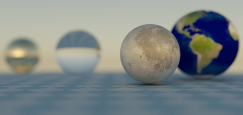
Finally, we need to actually use the textures in the materials. One easy way is to use a texture in place of a color in the material. For objects which just have a single color, like our gold orb, we can create a texture with one pixel.

1
2
3
4
5

struct Material {
    id: u32,
    desc: TextureDescriptor,
    x: f32,
}

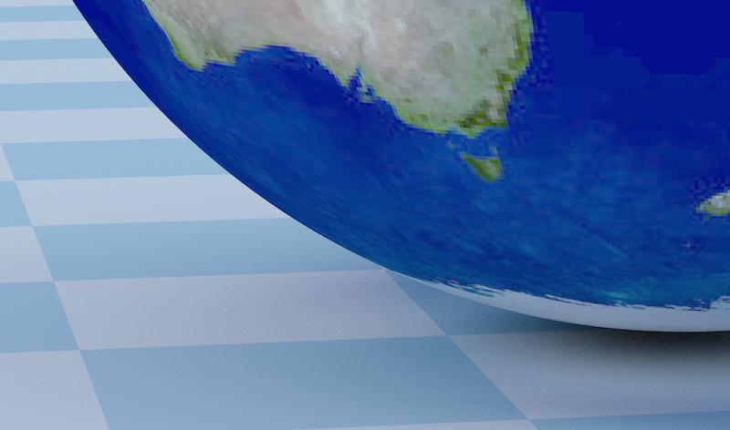
The drawback of this system is, of course, that we lose the built-in texture filtering abilities that WGSL provides. This is particularly visible when zooming in close to either the Moon or Earth.

Adding a checkerboard material

One final addition from the Ray Tracing: The Next Week book is the checkerboard material. We use two colors (two textures), and pick them depending on where we are on the surface. Two colors requires two textures descriptors, so our material declaration actually ends up being:

1
2
3
4
5
6

struct Material {
    id: u32,
    desc1: TextureDescriptor,
    desc2: TextureDescriptor,
    x: f32,
}

The checkerboard material’s scattering function multiplies the sines of the surface coordinate together, and uses that as a test for which checkerboard element we are in:

 1
 2
 3
 4
 5
 6
 7
 8
 9
10
11
12

fn scatterCheckerboard(rayIn: Ray, hit: Intersection, material: Material, rngState: ptr<function, u32>) -> Scatter {
    let sines = sin(5f * hit.p.x) * sin(5f * hit.p.y) * sin(5f * hit.p.z);
    var albedo: vec3<f32>;
    if sines < 0f {
        albedo = textureLookup(material.desc1, hit.u, hit.v);
    } else {
        albedo = textureLookup(material.desc2, hit.u, hit.v);
    }

    let scatterDirection = hit.n + rngNextVec3InUnitSphere(rngState);
    return Scatter(Ray(hit.p, scatterDirection), albedo);
}

References and links

weekend-raytracer-wgpu (project repository, see src/raytracer/raytracer.wgsl for full implementation)

Hosek-Wilkie sky model paper

hw-skymodel crate

glsl-tone-map

Ray Tracing: The Next Week