In inverse transform sampling, we use the inverse cumulative distribution function (CDF) to generate random numbers in a given distribution. But why does this work?
This post attempts to demystify inverse transform sampling works by plugging samples from a distribution into the same distribution’s CDF and verifying that we get numbers with a uniform distribution in \([0, 1]\).
Let’s start with a few definitions first.
Definitions
We want to generate random numbers according to a given probability density function (PDF) \(f(x)\). The probability density function \(f(x)\) and the cumulative distribution function \(F(x)\) are related to each other by an integral:
$$ F(x) = \int f(x) dx $$
We can use this to calculate the CDF of a simple function, the uniform density function U in the interval \([0,1]\). In U, the probability density is constant everywhere in the interval:
$$ F_U(x) = \int cdx = cx+d $$
The cumulative distribution function has the property that it must be zero before the range, and one after the range. We can use these constraints, \(U(0)=0\) and \(U(1)=1\), to obtain
$$ F_U(x) = x. $$
The CDF of a sample is uniformly distributed
Inverse transform sampling works, because when we plug values of random variable \(X\) into its own CDF \(F_X\), we obtain numbers which are uniformly distributed in \([0, 1]\). I.e., the shape of \(F_X(X)\) is uniform.
Let’s observe the distribution we obtain from the normal distribution’s CDF over normally distributed random numbers. This is easy to do with Python and a few libraries.
|
|
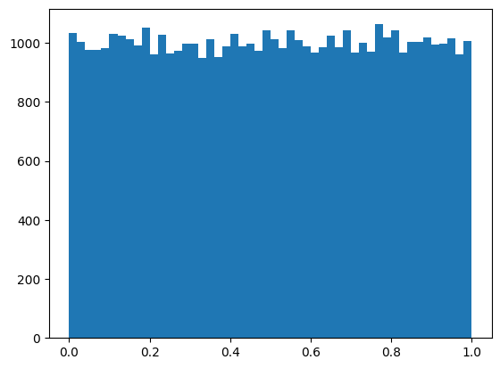
Histogram of normally distributed random numbers.
From the histogram we can see that \(F_N(N)\) yields nice uniformly distributed values between 0 and 1.
Using the definition of the CDF,
$$ F_X(x) = P(X \le x), $$
we also arrive at the conclusion that the distribution of \(F_X(X)\) is uniform. Let’s assign \(Z = F_X(X)\) and use the definition of the CDF on it:
$$ F_Z(x) = P(F_X(X) \le x) = P(F^{-1}_{X}(F_X(X)) \le F_X^{-1}(x)) = P(X \le F_X^{-1}(x)) $$
$$ \therefore F_Z(x) = F_X(F_X^{-1}(x)) = x $$
The shape of \(F_Z\) is that of the uniform distribution \(F_U\) that we calculated earlier! This is why for \(X\), our random number with a distribution, we can do this:
$$ F_X(X) = (\textrm{uniformly distributed number}) $$
$$ \therefore X = F^{-1}(\textrm{uniformly distributed number}). $$
Generating random numbers using inverse transform sampling
We can now generate random numbers in the shape of any given density function using the recipe:
- Given a PDF, calculate the CDF using the integral equation.
- Take the inverse of the CDF.
- Plug your uniformly distributed random numbers into the inverse CDF.
For example, to generate random numbers according to the density function \(f(x)=x^2\), in the range \([0,2]\), we can apply the recipe as follows.
First, we obtain the CDF.
$$ F(x) = \int x^2dx = C \frac{x^3}{3} $$
Using the constraints \(F(0)=0\) and \(F(2)=1\), we get
$$ F(x) = \frac{1}{8}x^3. $$
Next, let’s take the inverse of \(F(x)\):
$$ F^{-1}(x) = (8x)^{\frac{1}{3}} $$
Finally, we can plug numbers into our inverse function.
|
|

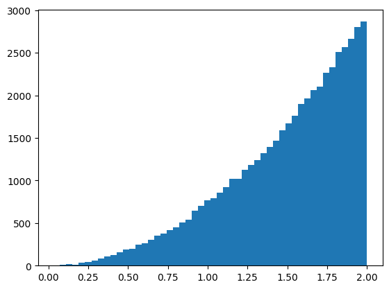
Histogram of random numbers sampled from the inverse of \\(x^2\\).
To confirm that everything works, we can look at a plot of \(x^2\).
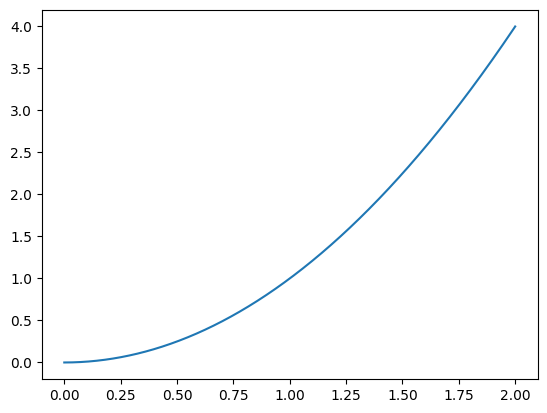
\\(x^2\\) as a curve.
Inverse transform sampling using normally distributed random numbers
The fact that evaluating a uniform distribution function yields uniformly distributed values means that we can actually plug in random numbers from any distribution into \(F^{-1}\)! Given that two CDFs \(F(X)\) and \(G(Y)\) have the exact same uniform distribution, we can apply the inverse of \(F^{-1}\) like we did before to find the mapping between \(X\) and \(Y\):
$$ F(X) = G(Y) $$
$$ \therefore X = F^{-1}(G(Y)) $$
We can use this fact to generate random numbers in our earlier distribution \(f(x)=x^2\) using normally distributed random numbers:
|
|
Histogram of random numbers sampled from the inverse of \\(x^2\\), using normally distributed random numbers.
And again, looks like a graph of \(x^2\)!
I’m not sure why you would want to generate random numbers in a given distribution in such a contrived way, but it’s nice to know that it is possible.